
A Full Guide to Risk Management
Everything you need to know about risk management


This is gonna be by far my biggest article, with the notebook from the risk manager that this was created with containing 1400+ lines of code and tons of visualizations! Actual risk management goes far beyond a stop loss order.
This article will cover both theory and practical applications that are often overlooked like taking into account liquidity.
I recommend you to copy the code into a jupyter notebook and play around with it as you read the article. There are a lot of important details in the code!
Table of Content
Risk Metrics
Volatility Modeling
Dependence Modeling
Stress Testing and Scenario Analysis
Liquidity-adjusted Value-at-Risk (LVaR) and Liquidity Modeling
Portfolio Optimization Under Tail Constraints
Final Remarks
Risk Metrics
Risk metrics exists to measure risk in some way. One takes into account tail-risk more than the other while others are usually more robust. Let’s go over the most important ones.
Value at Risk (VaR)
Value at Risk tells you the maximum potential loss over a specified time horizon at a given confidence level alpha, which is typically 95% or 99%.
Expressing this mathematically, VaR is defined as the quantile of the loss distribution:

Here L is the loss random variable and P is its probability measure.
This is obviously a very simple metric and because we are just looking at the specified quantile it fails to capture tail risk beyond that quantile. It’s also not subadditive, which can lead to counterintuitive results when aggregating risks across portfolios.
You can also do the parametric approach where you specify the distribution of the returns. If we assume that returns follow a normal distribution we then get the following formula:

Where mu and sigma are the mean and standard deviation of our normal distribution and Phi is the cumulative distribution function of the standard normal distribution. This will obviously underestimate tail risk even more since returns have much fatter tails than a normal distribution.
Expected Shortfall and Conditional Value at Risk
Expected Shortfall (ES), also known as Conditional Value at Risk (CVaR), does a much better job at assessing tail risk than VaR by measuring the expected loss beyond the VaR threshold:

This risk metric is also subadditive and even coherent which means that it is:
Normalized: ES(0) = 0
Monotonic: L_1 <= L_2 implies ES(L_1) >= ES(L_2)
Sub-additivity: ES(L_1 + L_2) <= ES(L_1) + ES(L_2)
Positive homogeneity: ES(a * L) = a * ES(L), where a >= 0
Translation invariance: If A is a deterministic portfolio with guaranteed return a then ES(L + A) = ES(L) - a
Where L, L_1, L_2 are losses. Note that sub-additivity and positive homogeneity together are equivalent to convexity.
We can also express CVaR as:

Now first let’s import all of the libraries we are gonna need in this article:
import numpy as np
import matplotlib.pyplot as plt
import pandas as pd

from scipy import stats
from scipy.stats import skew, kurtosis, gaussian_kde, t
from scipy.optimize import minimize
from scipy.linalg import cholesky
from sklearn.mixture import GaussianMixture
from statsmodels.tsa.stattools import acf

from arch import arch_model

import cvxpy as cp

from datetime import datetime, timedelta
import warnings
import hashlib
Here are the functions for computing logarithmic returns, VaR and CVaR:
def calculate_returns(prices):
    """
    Calculate logarithmic returns from price series

    Parameters:
    prices (pd.Series): Price series

    Returns:
    pd.Series: Log returns
    """
    return np.log(prices / prices.shift(1)).dropna()

def parametric_var(returns, confidence_level=0.05):
    """
    Calculate parametric VaR assuming normal distribution

    Parameters:
    returns (pd.Series): Return series
    confidence_level (float): Confidence level (default 5% for 95% VaR)

    Returns:
    float: VaR value
    """
    mean_return = returns.mean()
    std_return = returns.std()
    var = mean_return + std_return * stats.norm.ppf(confidence_level)
    return float(var)

def historical_var(returns, confidence_level=0.05):
    """
    Calculate historical VaR using empirical quantiles

    Parameters:
    returns (pd.Series): Return series
    confidence_level (float): Confidence level

    Returns:
    float: VaR value
    """
    return float(returns.quantile(confidence_level))

def expected_shortfall(returns, confidence_level=0.05):
    """
    Calculate Expected Shortfall (Conditional VaR)

    Parameters:
    returns (pd.Series): Return series
    confidence_level (float): Confidence level

    Returns:
    float: ES value
    """
    var = historical_var(returns, confidence_level)
    es = float(returns[returns <= var].mean())
    return es
Let us load in some data, run those functions and create some visualizations:
btc_prices = pd.read_csv("C:/QuantData/Klines/Perps/Binance/BTCUSDT.csv").set_index("timestamp")["close"] # You would use a different directory
btc_prices.index = pd.to_datetime(btc_prices.index*1000000)
btc_prices = btc_prices.resample("D").last()
btc_returns = calculate_returns(btc_prices)
# Calculate risk metrics
var_95 = historical_var(btc_returns, 0.05)
var_99 = historical_var(btc_returns, 0.01)
es_95 = expected_shortfall(btc_returns, 0.05)
es_99 = expected_shortfall(btc_returns, 0.01)
print(f"95% VaR: {var_95:.4f} ({var_95*100:.2f}%)")
print(f"99% VaR: {var_99:.4f} ({var_99*100:.2f}%)")
print(f"95% Expected Shortfall: {es_95:.4f} ({es_95*100:.2f}%)")
print(f"99% Expected Shortfall: {es_99:.4f} ({es_99*100:.2f}%)")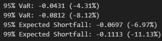
# Create a figure with two subplots
fig, (ax1, ax2) = plt.subplots(2, 1, figsize=(12, 8), height_ratios=[2, 1])
fig.suptitle('Bitcoin Price and Risk Metrics Analysis', fontsize=16)

# Plot 1: Price data
ax1.plot(btc_prices.index, btc_prices, label='BTC Price', color='blue')
ax1.set_ylabel('Price (USD)')
ax1.set_title('Bitcoin Price History')
ax1.grid(True)
ax1.legend()

# Plot 2: Returns with VaR and ES levels
ax2.plot(btc_returns.index, btc_returns, label='Daily Returns', color='gray', alpha=0.5)
ax2.axhline(y=var_95, color='red', linestyle='--', label=f'95% VaR: {var_95:.4f}')
ax2.axhline(y=var_99, color='darkred', linestyle='--', label=f'99% VaR: {var_99:.4f}')
ax2.axhline(y=es_95, color='orange', linestyle=':', label=f'95% ES: {es_95:.4f}')
ax2.axhline(y=es_99, color='darkorange', linestyle=':', label=f'99% ES: {es_99:.4f}')
ax2.set_ylabel('Log Returns')
ax2.set_title('Daily Returns with Risk Metrics')
ax2.grid(True)
ax2.legend()

# Adjust layout and display
plt.tight_layout()
plt.show()

# Print some additional statistics
print("\nAdditional Statistics:")
print(f"Mean Return: {float(btc_returns.mean()):.4f}")
print(f"Return Volatility: {float(btc_returns.std()):.4f}")
print(f"Skewness: {float(btc_returns.skew()):.4f}")
print(f"Kurtosis: {float(btc_returns.kurtosis()):.4f}")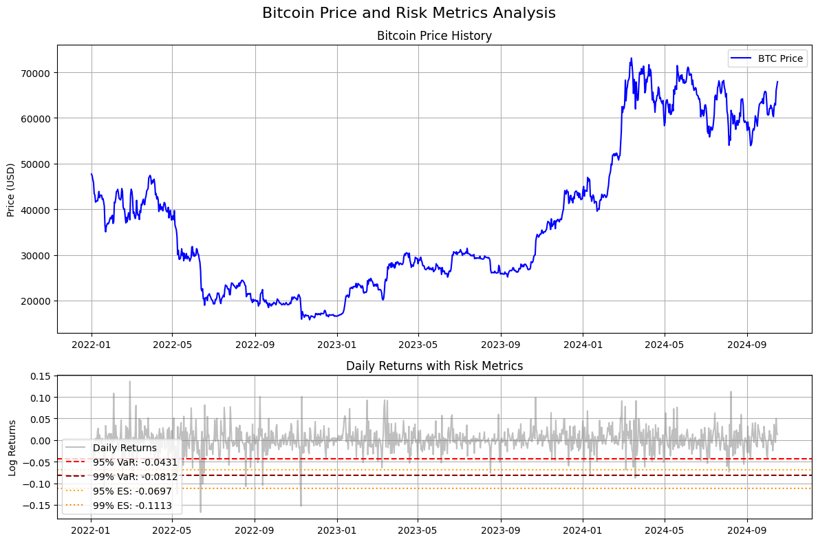
From all of this we see that:
Mean daily return of 0.03% (slightly positive)
Volatility of 2.87% which is high and typical for Bitcoin
Negative skewness (-0.2277) suggests that Bitcoin returns have a longer left tail, so extreme negative returns are more common than extreme positive returns
Kurtosis of 4.3779 suggests Bitcoin returns have heavier tails than a normal distribution which has a kurtosis of 3
95% VaR of -4.31% means that on any given day there’s a 95% chance that the loss won’t exceed 4.31%
99% VaR of -8.12% means that on any given day there’s a 99% chance that the loss won’t exceed 8.12% but also that losses can realistically get this bad
The ES values of -6.97% for the 95% confidence interval and -11.13% for the 99% condifence interval respectively indicate that when losses do exceed the VaR thresholds, they tend to be quite severe
# Visualization of VaR and ES
plt.figure(figsize=(15, 10))
# Plot 1: Return distribution with VaR and ES
plt.subplot(2, 2, 1)
plt.hist(btc_returns, bins=100, alpha=0.7, density=True, color='lightblue', edgecolor='black')
plt.axvline(var_95, color='red', linestyle='--', linewidth=2, label=f'95% VaR: {var_95:.3f}')
plt.axvline(var_99, color='darkred', linestyle='--', linewidth=2, label=f'99% VaR: {var_99:.3f}')
plt.axvline(es_95, color='orange', linestyle='-', linewidth=2, label=f'95% ES: {es_95:.3f}')
plt.axvline(es_99, color='darkorange', linestyle='-', linewidth=2, label=f'99% ES: {es_99:.3f}')
plt.xlabel('Daily Returns')
plt.ylabel('Density')
plt.title('BTC Return Distribution with Risk Metrics')
plt.legend()
plt.grid(True, alpha=0.3)
# Plot 2: Time series of returns with VaR and ES violations
plt.subplot(2, 2, 2)
plt.plot(btc_returns.index, btc_returns, alpha=0.6, color='blue', linewidth=0.5)
plt.axhline(var_95, color='red', linestyle='--', label='95% VaR')
plt.axhline(var_99, color='darkred', linestyle='--', label='99% VaR')
plt.axhline(es_95, color='orange', linestyle='-', label='95% ES')
plt.axhline(es_99, color='darkorange', linestyle='-', label='99% ES')
# Highlight VaR violations
violations_95 = btc_returns[btc_returns < var_95]
violations_99 = btc_returns[btc_returns < var_99]
plt.scatter(violations_95.index, violations_95, color='red', alpha=0.7, s=10, label='95% VaR Violations')
plt.scatter(violations_99.index, violations_99, color='darkred', alpha=0.7, s=10, label='99% VaR Violations')
plt.xlabel('Date')
plt.ylabel('Daily Returns')
plt.title('BTC Returns with Risk Metrics and Violations')
plt.legend()
plt.grid(True, alpha=0.3)
plt.xticks(rotation=20)
plt.show()
# Calculate violation rates
violation_rate_95 = len(violations_95) / len(btc_returns)
violation_rate_99 = len(violations_99) / len(btc_returns)
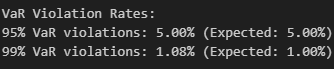
print(f"\nVaR Violation Rates:")
print(f"95% VaR violations: {violation_rate_95:.2%} (Expected: 5.00%)")
print(f"99% VaR violations: {violation_rate_99:.2%} (Expected: 1.00%)")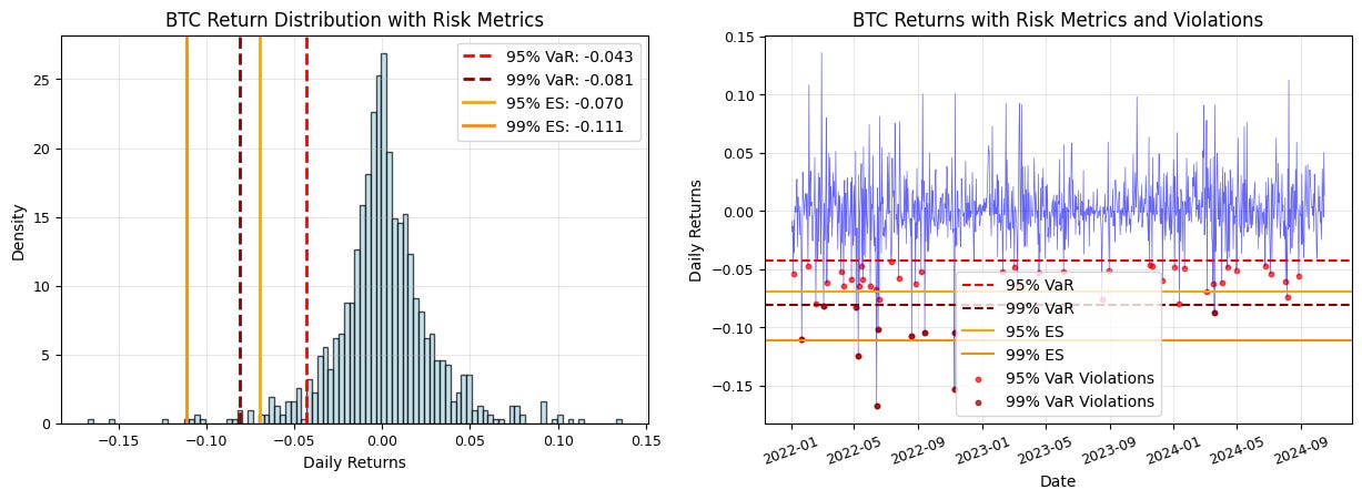
You can notice that the violations (when loss exceeds the VaR levels) cluster during volatile periods.
The plot on the right helps you visualize:
How often violations occur
The magnitude of the violations (Also seen from the distance between the ES and VaR lines)
Any potential regime changes in the risk profile
Maximum Drawdown
Maximum Drawdown (MDD) measures the largest loss from a peak to a trough over a specified period. This risk metric is basically always looked at and tells you a lot about how stable and sustainable a strategy is and what you can expect in the worst-case scenario (although you should always expect even worse). Mathematically we can formula it as:

where P_t is the portfolio value at time t.
While VaR and ES focus on single-period risks, maximum drawdown captures the cumulative effect of sustained negative performance, making it more relevant for evaluating long-term investment strategies. Besides the maximum drawdown you could also look at the average of all drawdowns above a certain threshold and other similar metrics.
Other important values in drawdown analysis are also the drawdown duration and recovery time. The drawdown duration measures how long it takes for a portfolio to return to its previous peak. Recovery time measured the time required to reach new highs.
Here is the code for calculating drawdowns, drawdown duration, max drawdown etc:
def calculate_drawdown_series(prices):
    """
    Calculate drawdown series from price data

    Parameters:
    prices (pd.Series): Price series

    Returns:
    pd.DataFrame: DataFrame with peak, drawdown, and duration information
    """

    # Calculate running maximum (peak)
    peak = prices.expanding().max()

    # Calculate drawdown
    drawdown = (prices - peak) / peak

    # Calculate drawdown duration
    duration = np.zeros(len(drawdown))
    current_duration = 0

    for i in range(len(drawdown)):
        if float(drawdown.iloc[i]) < 0:  # Convert to float for comparison
            current_duration += 1
        else:
            current_duration = 0
        duration[i] = current_duration

    return pd.DataFrame({
        'Price': prices,
        'Peak': peak,
        'Drawdown': drawdown,
        'Duration': duration
    })

def calculate_max_drawdown_stats(drawdown_series):
    """
    Calculate maximum drawdown statistics

    Parameters:
    drawdown_series (pd.DataFrame): Output from calculate_drawdown_series

    Returns:
    dict: Dictionary with MDD statistics
    """
    max_dd = drawdown_series['Drawdown'].min()
    max_dd_date = drawdown_series['Drawdown'].idxmin()
    max_duration = drawdown_series['Duration'].max()

    # Find the peak before maximum drawdown
    peak_before_mdd = drawdown_series.loc[:max_dd_date, 'Peak'].iloc[-1]
    peak_date = drawdown_series.loc[:max_dd_date, 'Peak'].idxmax()

    return {
        'max_drawdown': max_dd,
        'max_drawdown_date': max_dd_date,
        'peak_before_mdd': peak_before_mdd,
        'peak_date': peak_date,
        'max_duration': max_duration
    }
Trying it on our data:
btc_drawdown = calculate_drawdown_series(btc_prices)
mdd_stats = calculate_max_drawdown_stats(btc_drawdown)

# Print statistics
print(f"Maximum Drawdown Statistics for BTC:")
print(f"Maximum Drawdown: {mdd_stats['max_drawdown']:.2%}")
print(f"Date of Maximum Drawdown: {mdd_stats['max_drawdown_date'].strftime('%Y-%m-%d')}")
print(f"Peak before MDD: ${mdd_stats['peak_before_mdd']:,.2f}")
print(f"Peak Date: {mdd_stats['peak_date'].strftime('%Y-%m-%d')}")
print(f"Maximum Duration: {mdd_stats['max_duration']:.0f} days")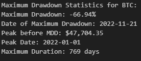
In our time interval from 2022-01-01 to 2024-10-16 we had a staggering -66.94% maximum drawdown. This went on from 2022-01-01 to 2022-11-21 starting at a price of $47,704.35 and lasting in total 769 days (approximately 2.3 years).
Note: The fact that maximum drawdown begins at the starting date of our data means that if we use data going back further the drawdown could potentially be even bigger.
This means taht if you were to invest in bitcoin you should be prepared for potential drawdowns of up to 70% or more.
Here we also have a visualization for the drawdown and volatility of Bitcoin:
# Create the visualization
plt.figure(figsize=(12, 8))

# Plot drawdown analysis
plt.subplot(2, 2, 3)
plt.fill_between(btc_drawdown.index, 0, btc_drawdown['Drawdown'],
                alpha=0.7, color='red', label='Drawdown')
plt.axhline(mdd_stats['max_drawdown'], color='darkred', linestyle='--',
           label=f'Max DD: {mdd_stats["max_drawdown"]:.1%}')
plt.xlabel('Date')
plt.ylabel('Drawdown')
plt.title('BTC Maximum Drawdown Analysis')
plt.legend()
plt.grid(True, alpha=0.3)
plt.xticks(rotation=20)

# Plot rolling volatility
plt.subplot(2, 2, 4)
rolling_vol = btc_returns.rolling(window=30).std() * np.sqrt(252)

plt.plot(rolling_vol.index, rolling_vol.values, color='purple', linewidth=1)
plt.fill_between(rolling_vol.index, 0, rolling_vol.values, alpha=0.3, color='purple')
plt.xlabel('Date')
plt.ylabel('Annualized Volatility')
plt.title('30-Day Rolling Volatility (Annualized)')
plt.grid(True, alpha=0.3)

plt.tight_layout()
plt.xticks(rotation=20)
plt.show()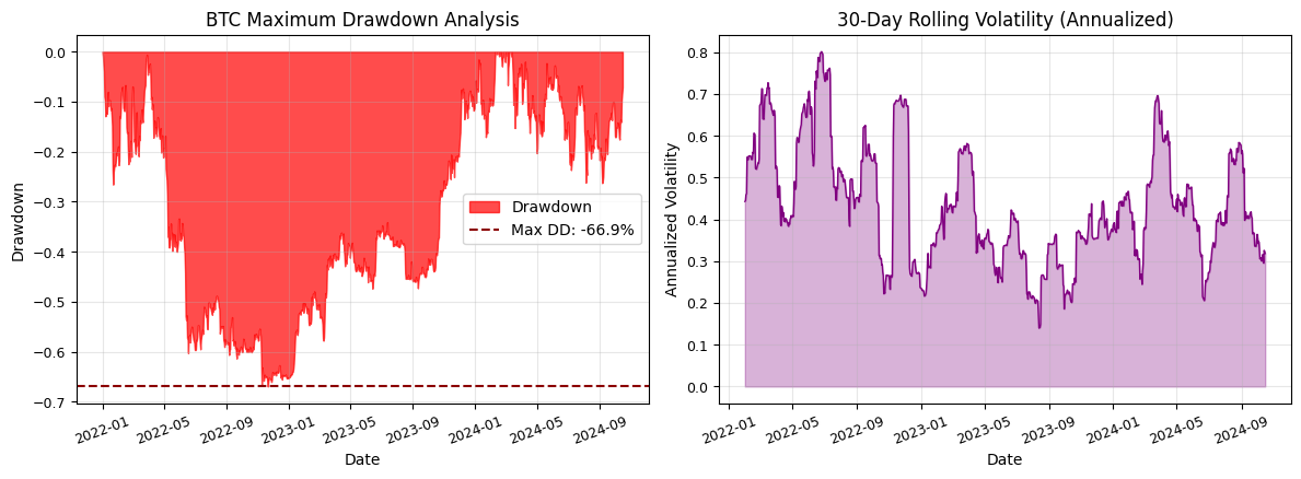
 | A guest post by
|