Are Greeks beyond the third order necessary?

How much you are missing by only using greeks up to third order

Most of the time we only use greeks up to the second order, maybe even third order but I’ve never seen someone use greeks beyond that. Is that just a bad convention that everyone assumes to be fine and those greeks do actually matter or is it fine to measure risk only up to at most 3rd order? That’s what we will explore in this article. On the Wikipedia page on greeks there are only a few 3rd order greeks mentioned and 4th order greeks are completely ignored:

https://en.wikipedia.org/wiki/en:Greeks_(finance)?variant=zh-tw

---

Table of Content

1. Where do Greeks come from?

2. Taylor Expansion

3. 1st-order Greeks Error Bounds

4. 2nd-order Greeks Error Bounds

5. Final Remarks

---

Where do Greeks come from?

Greeks appear from the Black-Scholes model so we first need to understand how that one works so I’m gonna give a very quick rundown:

Black-Scholes first assumes that prices follow a random random walk with constant drift and volatility and are therefore lognormally distributed.

The models price for a call option is:

where:

• Phi = CDF of the Normal Distribution

• S = Underlying Price

• K = Strike Price

• r = risk-free interest rate

• t = Time to maturity

• sigma = volatility

Sidenote: I recently visited a lecture by one of the creators of the Black-Scholes Merton Model, Robert C. Merton. He is an incredibly interesting and intelligent person!

Now when things like the underlying price or the volatility change then our call price will change as well. The greeks simply tell you how much the call price changes if you change one of the following: S, r, t, sigma. So they are nothing more than partial derivatives.

Here are the first order greeks:

Where small phi is the PDF of the normal distribution.

Notice how we put a negative sign for the Theta. This convention is used because you don’t go backwards in time and we wanna use a positive number for the passage of time instead of a negative number.

We will ignore rho and other greeks depending on interest rates in this article as the other ones are way more important.

For second-order greeks we will also only look at greeks where we differentiate with respect to the same variable twice for price and volatility:

And lastly the third order greeks that we care about:

Here is the code to calculate all of the greeks and option prices:

def d1(S, K, r, sigma, t):
    return (np.log(S/K) + (r + sigma**2 / 2)*t) / (sigma*np.sqrt(t))
def d2(S, K, r, sigma, t):
    return d1(S, K, r, sigma, t) - sigma*np.sqrt(t)
def C(S, K, r, sigma, t):
    return norm.cdf(d1(S, K, r, sigma, t))*S - norm.cdf(d2(S, K, r, sigma, t))*K*np.exp(-r*t)

def delta(S, K, r, sigma, t):
    return norm.cdf(d1(S, K, r, sigma, t))
def vega(S, K, r, sigma, t):
    return K*np.exp(-r*t)*norm.pdf(d2(S, K, r, sigma, t))*np.sqrt(t)
def theta(S, K, r, sigma, t):
    return -(S*norm.pdf(d1(S, K, r, sigma, t))*sigma)/(2*np.sqrt(t)) - r*K*np.exp(-r*t)*norm.cdf(d2(S, K, r, sigma, t))
def rho(S, K, r, sigma, t):
    return K*t*np.exp(-r*t)*norm.cdf(d2(S, K, r, sigma, t))

def gamma(S, K, r, sigma, t):
    return K*np.exp(-r*t)*norm.pdf(d2(S, K, r, sigma, t))/(S**2 * sigma * np.sqrt(t))
def vomma(S, K, r, sigma, t):
    return vega(S, K, r, sigma, t)*d1(S, K, r, sigma, t)*d2(S, K, r, sigma, t)/sigma

def speed(S, K, r, sigma, t):
    return -(gamma(S, K, r, sigma, t)/S)*(d1(S, K, r, sigma, t)/(sigma*np.sqrt(t)) + 1)
def ultima(S, K, r, sigma, t):
    d1_val = d1(S, K, r, sigma, t)
    d2_val = d2(S, K, r, sigma, t)
    return -(vega(S, K, r, sigma, t)/sigma**2)*(d1_val*d2_val*(1-d1_val*d2_val) + d1_val**2 + d2_val**2)

---

Taylor Expansion

We can write an infinitely differentiable function as an infinite sum of its derivatives around some point:

The notation here means that f^(n) is the n-th derivative and f^(0) = f.

Now imagine we broke this sum into 2 parts. One finite one up to N and the rest an infinite sum starting at N+1:

The left sum is the so called Nth order Taylor Polynomial and the right part the remainder:

It makes sense intuitively that as you increase N the Taylor Polynomial more and more accurately estimates our function f. We can say something really fascinating about the remainder:

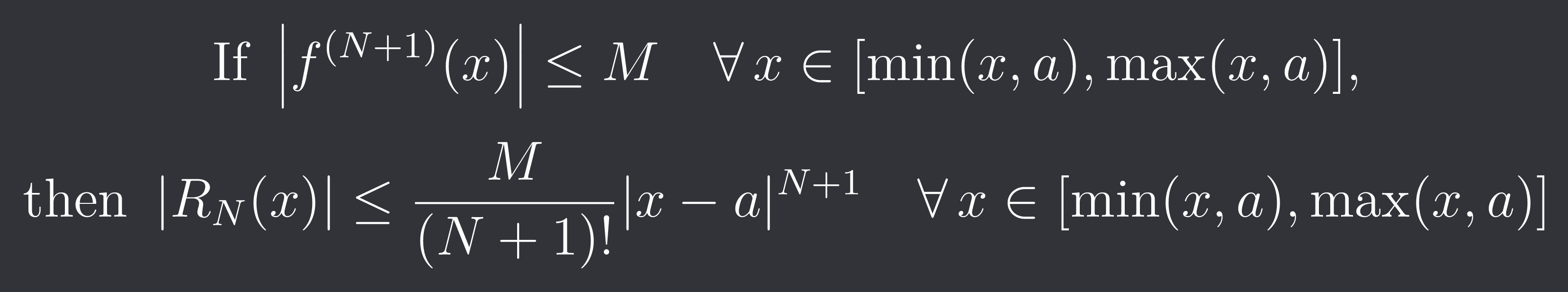
where xi is some value between x and a. The remainder therefore only depends on the derivative one order higher! If we can bound this derivative then we can also bound the remainder (error):

We can apply this to our call price now!

---

1st-order Greeks Error Bounds

For our analysis we will always look at 1 variable at a time because otherwise you need a multivariate taylor expansion, the visualization isn’t as nice anymore and it’s harder to interpret.

The first order taylor expansion and residual of call price against price is:

written with greeks:

delta S here stands for our change in S as we will do the taylor expansion around the current underlying price S. tilde S stands for some underlying price between S and S + delta S. We will continue using this notation for the other greeks as well.

So what we have to do now is get a list of prices we want to check and for each of those prices find the biggest absolute value of gamma between the current price and that price so that we can bound the error of our first order taylor expansion.

Note: We won’t be using any fancy optimization algorithms here to find the maxima of the greeks but just check a bunch of different values.

We will be using real BTC options data in the following example:

S = 105009.5
K = 100000
r = 0
sigma = 0.9251
t = 404.75/525600

price_change_range = np.linspace(-10000, 10000, 1000)

call_value_S0 = C(S, K, r, sigma, t)
delta_value_S0 = delta(S, K, r, sigma, t)

taylor_call_values = []
actual_call_values = []
upper_bounds = []
lower_bounds = []
for dS in price_change_range:
    taylor_call_values.append(call_value_S0 + delta_value_S0*dS)
    actual_call_values.append(C(S+dS, K, r, sigma, t))
    grid = np.linspace(min(S, S + dS), max(S, S + dS), 100)

    max_abs_higher_greek = max(abs(gamma(grid, K, r, sigma, t)))
    
    bound = 0.5 * max_abs_higher_greek * dS**2

    upper_bounds.append(taylor_call_values[-1]+bound)
    lower_bounds.append(taylor_call_values[-1]-bound)

plt.plot(price_change_range, actual_call_values, label='Actual Call Value', color='black', linewidth=2)
plt.plot(price_change_range, taylor_call_values, label='Taylor Approximation', color='blue', linestyle='--', linewidth=2)
plt.plot(price_change_range, upper_bounds, label='Upper Bound', color='green', linestyle=':', linewidth=1.5)
plt.plot(price_change_range, lower_bounds, label='Lower Bound', color='red', linestyle=':', linewidth=1.5)

plt.xlabel("Underlying Price Change")
plt.ylabel("Option Value")
plt.title("Call Option Value vs Taylor Approximation and Bounds")

plt.legend()
plt.grid(True, linestyle='--', alpha=0.6)

plt.tight_layout()
plt.show()

You can see how the taylor expansion becomes really inaccurate when price drops a ton but for small drops and relatively big increases it still stays relatively accurate!

Let’s do the same for the implied volatility now:

This one is inaccurate no matter where implied volatility goes.

Now while in practice you constantly reassess your risk and not just do it once you could still run into some problems if markets have a sudden shift.

Let’s move on to using a second order taylor expansion which (given the shape of those 2 curves) seems much more appropriate.

---

2nd-order Greeks Error Bounds

The second order taylor expansion with respect to price is:

And with respect to volatility:

Let’s get the same plots as before but now with the second order taylor expansions:

price_change_range = np.linspace(-10000, 10000, 1000)

call_value_S0 = C(S, K, r, sigma, t)
delta_value_S0 = delta(S, K, r, sigma, t)
gamma_value_S0 = gamma(S, K, r, sigma, t)

taylor_call_values = []
actual_call_values = []
upper_bounds = []
lower_bounds = []
for dS in price_change_range:
    taylor_call_values.append(call_value_S0 + delta_value_S0*dS + 0.5*gamma_value_S0*dS**2)
    actual_call_values.append(C(S+dS, K, r, sigma, t))

    grid = np.linspace(min(S, S + dS), max(S, S + dS), 100)
    max_abs_higher_greek = max(abs(speed(grid, K, r, sigma, t)))
    
    bound = 1/6 * max_abs_higher_greek * dS**3

    upper_bounds.append(taylor_call_values[-1]+bound)
    lower_bounds.append(taylor_call_values[-1]-bound)

plt.plot(price_change_range, actual_call_values, label='Actual Call Value', color='black', linewidth=2)
plt.plot(price_change_range, taylor_call_values, label='Taylor Approximation', color='blue', linestyle='--', linewidth=2)
plt.plot(price_change_range, upper_bounds, label='Upper Bound', color='green', linestyle=':', linewidth=1.5)
plt.plot(price_change_range, lower_bounds, label='Lower Bound', color='red', linestyle=':', linewidth=1.5)

plt.xlabel("Underlying Price Change")
plt.ylabel("Option Value")
plt.title("Call Option Value vs Taylor Approximation and Bounds")

plt.legend()
plt.grid(True, linestyle='--', alpha=0.6)

plt.tight_layout()
plt.show()

which is very similar to the first order taylor expansion because call value is mostly linear with respect to price around the current underlying price.

And for implied volatility:

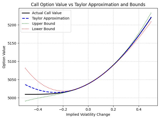
This is a MUCH better fit than before! Although it still seems to be a little inaccurate if IV drops a lot.

Lastly here is what the third order taylor polynomials look like:

---

Final Remarks

In this article we’ve figured out how to give hard bounds on the approximation of option price with greeks up to a certain order.

In reality you constantly reassess risk and with greeks up to second order we can capture the shape of call prices quite well for moderately small changes in price and volatility. This is the reason higher order greeks than that aren’t usually used!

You can do the same analysis for multiple conditions changing at once using multivariate taylor series and using the other greeks.

Discord: https://discord.gg/X7TsxKNbXg