In the previous article, we looked at latency arbitrage / lead-lag.
We went through the techniques commonly found in literature, starting from simple techniques like linear regression to more complex ones like looking for curvature in the shortest path of a distance matrix.
Latency Arbitrage - How to start
In the previous article, we looked at how to properly do DCA (Dollar-Cost-Averaging) by quantifying different approaches and seeing how they impact returns, variance and downside variance. In this article, we are gonna look at one of my favorite HFT trades: Lead Lag Arbitrage or Latency Arbitrage.
In this article, we are gonna learn about clustering algorithms and code up the k-means clustering algorithm from scratch.
The goal of this isn’t to get the best implementation of the algorithm (you would usually use libraries for that) but to understand the algorithms on a deeper level.
This sort of “practice” when it comes to learning such topics is incredibly valuable.
If you end up enjoying this article consider getting the paid sub, that way you can support me and I can write even more articles!
Here is a discount code for those interested: https://www.vertoxquant.com/62375e34
Table of Content
Applications of Clustering Algorithms
Types of Clustering Algorithms
k-means Clustering
DBSCAN
OPTICS
GMM
Hierarchical Clustering
Min-Max Distance Clustering
Dimensionality Reduction
Final Remarks
Applications of Clustering Algorithms
The first question you may ask yourself with all of this is: “What’s the point?”
The first thing that may come to mind to my readers is its use in statistical arbitrage strategies. Mean reverting portfolios, lead-lag (https://www.vertoxquant.com/p/latency-arbitrage-how-to-start) and other types of stat arbs.
In other words, it’s commonly used to find similar assets.
This is also often done in portfolio optimization, you wouldn’t want to diversify across assets in the same cluster, instead you would want to construct a portfolio consisting of assets from different portfolios.
Another more unique approach is segmenting variables into different behaviors.
For example: How does the market (returns) behave like for different levels of volatility?
One cluster could be a trending market and one a mean reverting one for example.
With this specific example, HMMs are commonly used but things like GMMs (Similar name but something different) can be used too.
Types of Clustering Algorithms
While not all clustering algorithms are the same some behave very similarly and work based on a similar concept.
Centroid-based
With centroid-based clustering algorithms, we find multiple centroids which are the centers of individual clusters. We then assign data points to different clusters based on the distance to the clusters’ centroid.
Distance-based
This is probably my favorite category. Dense areas of data points become clusters. This is the most flexible approach and also handles outliers well.
Distribution-based
Here each of our clusters is a probability distribution. That way we can assign a probability of a datapoint belonging to a distribution.
The big problem with this approach is that you have to assume a distribution for your clusters which is usually easier said than done.
Hierarchical
With this one, we create a tree-like hierarchy of our data points. The same way a tree branches out so do our clusters with bigger clusters containing smaller clusters.
Graph-based
With graph-based clustering approaches, we make our data points form a graph, the nodes being the data points themselves and the edges being the distances/relationships between our data points. We can then apply different techniques from graph theory to find clusters.
If you need a refresher on graph theory I have a little crash course thread on my Twitter/X: https://twitter.com/Vertox_DF/status/1682323985961308160
k-means clustering
Before we look into k-means clustering let’s write a script that will generate multiple random clusters for us.
We will do it the following way:
Pick k random points in a [0,1] x [0,1] area, those will be the centers of our clusters.
For each center, we generate a normal distribution with a standard deviation somewhere between 0.01 and 0.1.
For each distribution, we generate n data points.
def generate_data(k, n):
    points = np.random.rand(k, 2)

    scales = np.random.uniform(0.01, 0.1, size=k)

    data = np.concatenate([np.random.normal(loc=point, scale=scale, size=(n, 2)) for point, scale in zip(points, scales)])

    return data
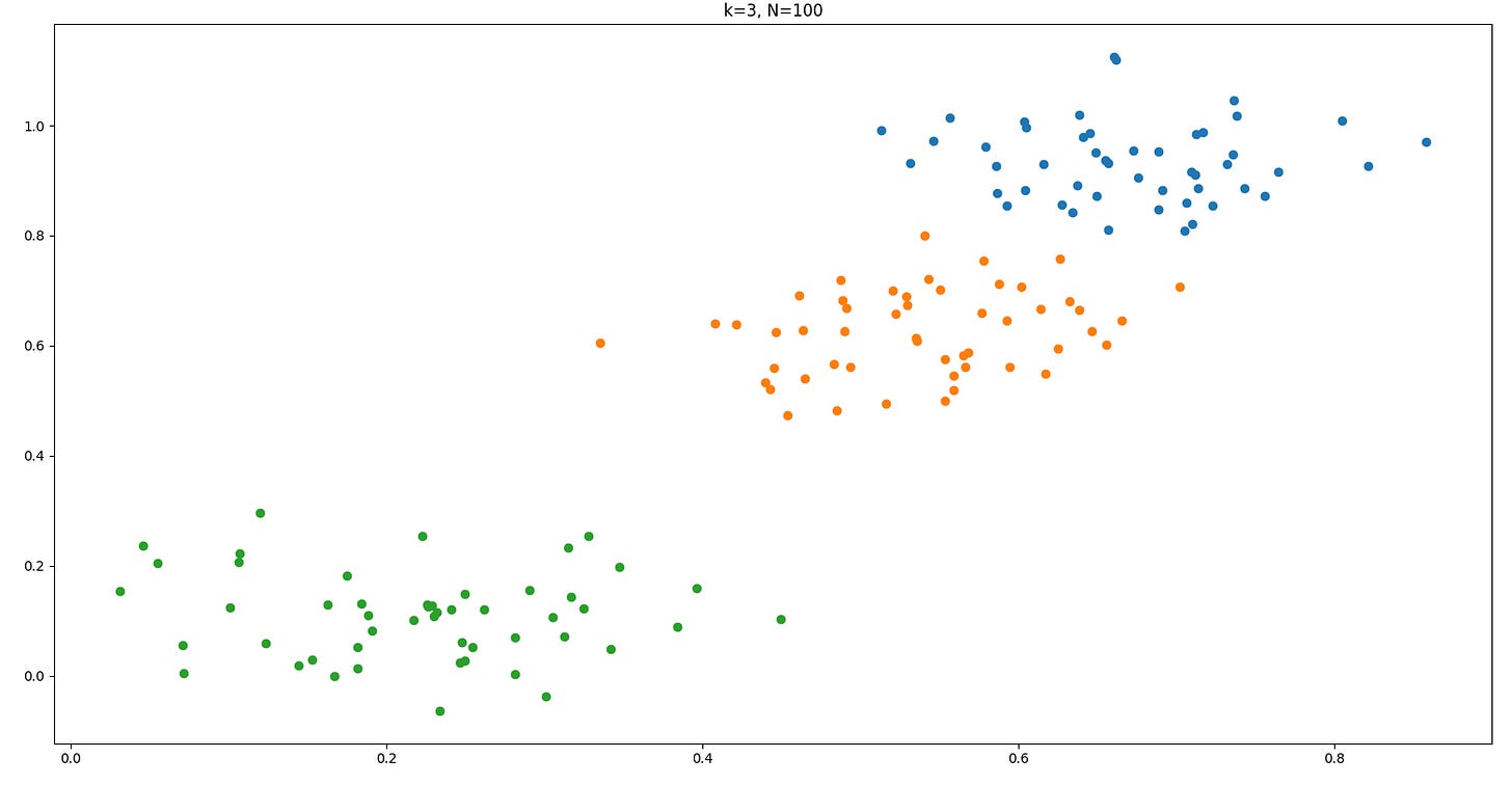
Here is one example we get for generate_data(3, 100)
With that out of the way let us now look at the first clustering algorithm: k-means clustering, a centroid-based clustering algorithm.
Select the number k of clusters you want to identify.
Randomly select k random data points and set them as individual clusters.
Measure the distance between the first datapoint and our k clusters.
Assign the first data point to the nearest cluster.Repeat step 3 until all data points are assigned to a cluster.
The first 4 steps may result in something like this:
Calculate the mean of each cluster.
Measure the distance of each data point to the means of the clusters.
Assign the data point to the nearest cluster.If no data point got re-assigned to a new cluster in step 6: terminate.
Otherwise: Repeat steps 5 and 6.
Doing this for our example above yields the following:
And now our algorithm terminates because the clusters didn’t change.
That is a pretty horrible result though.
K-Means clustering goes 1 step further to prevent results like this:
Get the total sum of distances of data points from their cluster means.
Rerun the algorithm N times and pick the result with the lowest sum of distances.
Let us code this up now!
First, we need a function to get the distance between 2 points. We are gonna use simple euclidian distance for that:
def distance(point1, point2):
    return math.sqrt((point1[0]-point2[0])*(point1[0]-point2[0]) + (point1[1]-point2[1])*(point1[1]-point2[1]))
Now we can code the algorithm itself.
Here are the first 4 steps coded up:
def k_means(k, N, data):
    clusters = [[] for _ in range(k)]
    cluster_means = []

    # Pick k random starting points
    selected_indices = np.random.choice(len(data), size=3, replace=False)
    selected_points = data[selected_indices]

    for i in range(k):
        clusters[i].append(selected_points[i])
        cluster_means.append(selected_points[i])

    data = np.delete(data, selected_indices, axis=0)

    # Keep picking points and assigning them to clusters
    while len(data) > 0:
        next_indice = np.random.choice(len(data), size=1)
        next_point = data[next_indice][0]

        data = np.delete(data, next_indice, axis=0)

        # Find closest cluster
        best_index = 0
        best_distance = distance(next_point, cluster_means[0])
        for i in range(1, k):
            new_distance = distance(next_point, cluster_means[i])

            if new_distance < best_distance:
                best_distance = new_distance
                best_index = i

        clusters[best_index].append(next_point)


    for i in range(k):
        plt.scatter(np.array(clusters[i])[:, 0], np.array(clusters[i])[:, 1])

    return clusters
And here is the entire algorithm:
def k_means_single(data, k: int):
    clusters = [[] for _ in range(k)]
    cluster_means = []

    # Pick k random starting points
    selected_indices = np.random.choice(len(data), size=k, replace=False)
    selected_points = data[selected_indices]

    for i in range(k):
        clusters[i].append(selected_indices[i])
        cluster_means.append(selected_points[i])

    # Keep picking points and assigning them to clusters
    for i in range(len(data)):
        if i not in selected_indices:
            next_point = data[i]

            # Find closest cluster
            best_index = 0
            best_distance = distance(next_point, cluster_means[0])
            for j in range(1, k):
                new_distance = distance(next_point, cluster_means[j])

                if new_distance < best_distance:
                    best_distance = new_distance
                    best_index = j

            clusters[best_index].append(i)

    old_clusters = clusters

    # Reassign data points to new clusters
    while True:
        new_clusters = [[] for _ in range(k)]

        # Calculate Means
        for i in range(k):
            cluster_means[i] = [np.mean([data[idx][0] for idx in old_clusters[i]]), np.mean([data[idx][1] for idx in old_clusters[i]])]


        # Keep picking points and assigning them to clusters
        for i in range(len(data)):
            next_point = data[i]

            # Find closest cluster
            best_index = 0
            best_distance = distance(next_point, cluster_means[0])
            for j in range(1, k):
                new_distance = distance(next_point, cluster_means[j])

                if new_distance < best_distance:
                    best_distance = new_distance
                    best_index = j

            new_clusters[best_index].append(i)

        if new_clusters == old_clusters:
            break

        old_clusters = new_clusters


    # Calculate total variation of clusters
    variation = 0

    for i in range(len(new_clusters)):
        for idx in new_clusters[i]:
            variation += distance(data[idx], cluster_means[i])

    return new_clusters, variation
def k_means(data, k: int, N: int, plot: bool):
best_cluster = []
best_variation = float('inf')
# Run k_means algorithm N times and return the best result
for _ in range(N):
next_cluster, next_variation = k_means_single(data, k)
if next_variation < best_variation:
best_variation = next_variation
best_cluster = next_cluster
# Plot result
if plot:
for i in range(len(clusters)):
plt.scatter([datapoints[idx][0] for idx in clusters[i]], [datapoints[idx][1] for idx in clusters[i]])
plt.title(f"k={k}, N={N}")
plt.show()
return best_cluster, best_variationAnd here is one results for k=3 and N=100:
Now for this dataset, the k we should pick is quite obvious but this is often not the case in reality.
There is 1 trick we can use to figure out the optimal k though, the so-called “Elbow-Method”.
We simply run the algorithm for different values of k and plot the variation for each number of clusters.
The elbow of this plot will then be a good middle ground.
Here is what that looks like for our specific example:
The elbow is at k=3 just like we expected.
DBSCAN
DBSCAN stands for Density-Based Spatial Clustering of Applications with Noise and is a density-based clustering algorithm.
Imagine you have the following dataset:
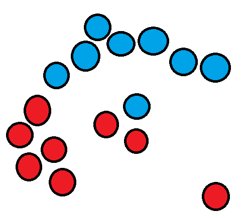
We couldn’t use k-means clustering in this case as the long cluster wraps around the smaller cluster and the centroids would overlap.
If we ran k-means with k=2 here we may get something like this as a result:
This is not what we want, the outlier also doesn’t seem to belong to the 2 clusters, in scenarios like this we need a more flexible clustering algorithm like DBSCAN.
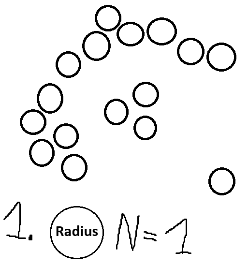
Pick a radius and a number N.
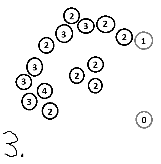
For each point, check how many close points it has (points within its radius).
Each point that has more than N close points becomes a core point.
Randomly pick a core point and assign it to a cluster.
Close core points of the cluster become assigned to the cluster.
Once there are no more close core points, assign the close regular points to the cluster.
Go back to step 4 and repeat until there are no more core points that don’t belong to a cluster.
Any leftover points not assigned to clusters are outliers.
Here is what that would look like for our dataset above:
And with that, we are done. The white points (in our case the point to the bottom right) are outliers.
As you can probably tell this algorithm is really sensitive to the initial parameters if you don’t have very distinct clusters.
Here is something that can happen if your radius is too small and/or your N is too small:
And here is something that can happen if your radius is too small and/or your N is too big:
OPTICS
There is one more really big disadvantage to DBSCAN. It doesn’t work well if your clusters have different densities like in this example:
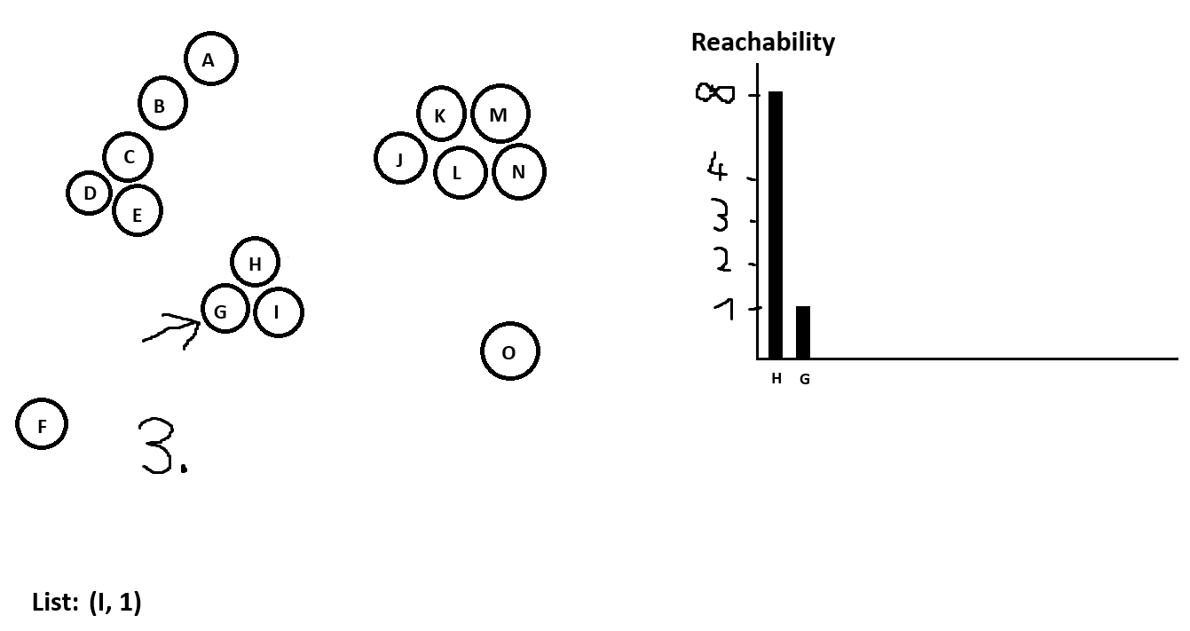
OPTICS, which stands for “Ordering Points To Identify Clustering Structure”, tries to solve this problem by instead of having a fixed radius we now have a fixed maximum radius instead and can use any radius between 0 and the maximum radius.
Before we dive into the algorithm let’s define 2 new concepts:
Core Distance
The core distance of a core point p is the minimum radius at which p is still a core point (More than N other points within its core distance).
If p isn’t a core point then the core distance would have to be bigger than the maximum radius which we do not allow so we would set the core distance as undefined.
Reachability Distance
The reachability distance of a point p to a core point q is defined as:
max(core-distance(q), distance(p, q))
And once again if the reachability distance would be bigger than the maximum radius (if the distance between p and q is bigger than the maximum radius of q, in which case q is not reachable from p) then it’s also undefined.
Now let’s see how the algorithm works.
Pick a maximum radius and a number N.
Pick a random point p and put its neighbors with their reachability distances into a list. Set the reachability distance of p to infinite and add it to the reachability plot.
Go to the next point in the list, add its neighbors to the list or update them if they are already in the list and the reachability distance becomes smaller. Sort the list in increasing order by reachability distance. Add the current point in the reachability plot.
If our list is not empty go back to step 3.
If we haven’t visited all points yet go back to step 2. If we already visited all points terminate and identify the clusters using the reachability plot.
Let’s look at an example:
Our list is empty now but we have not visited all points yet so we pick a random point again.
If we keep running this algorithm until we go through all points we are gonna be left with a reachability plot that will look something like this:
There are multiple ways to identify clusters in this algorithm now, here is one of them:
Identify outliers. Those could be all points with infinite reachability distance.
Set the first point in the reachability plot as a cluster.
Go to the next point.If there is a sharp increase in reachability we start a new cluster.
If there is an outlier we skip it.
Else assign the current point to the current cluster.
Repeat.
This would result in the following:
Identifying clusters from the reachability plot is its very own rabbit hole.
GMM
This is our first distribution-based clustering technique and as the name implies it uses a multivariate Gaussian distribution for each cluster.
The multivariate Gaussian distribution is defined in the following way:
where Sigma is the covariance matrix and mu is the mean of the distribution.
As the name implies we have a mixture of Gaussians.
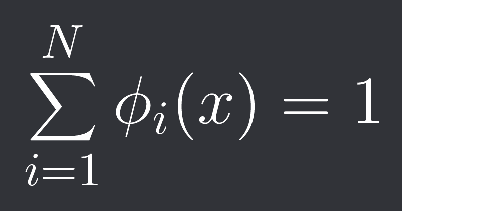
We are gonna define the probability of a datapoint x belonging to cluster i as phi_i(x).
The constraint is:
where N is our number of clusters, so the total probability distribution gets normalized.
We can then get the probability of data point x being observed as:
The goal of GMM is to find the best Sigma and mu for each cluster.
This is done via Expectation-Maximization (EM).
Initialization step:
Set the means mu_1, …, mu_N to randomly picked data points.
Set the covariances Sigma_1, …, Sigma_N to the sample covariance.
where M is our total number of data points, x_hat is the x coordinate of data point x, y_hat is the y coordinate of data point x, x_bar is the mean of x coordinates and y_bar is the mean of y coordinates.
Set the phis to the uniform distribution.Expectation Step:
Calculate all the probabilities of data point i belonging to cluster k as:
(This is derived via Bayes theorem for those wondering)
Maximization Step:
Update your phis, Sigmas and mus as follows:where mu_bar_j stands for the mean of the j-th cluster.
This is derived by maximizing the total probability of observing all data points by taking the derivative with respect to the 3 parameters and setting it to 0.The total probability of observing all data points is simply the probabilities of observing the individual data points multiplied since they are assumed to be independent.
We then keep repeating step 2 and 3 until we have a result that satisfies us.
Just like with k-means clustering we would try out different values N for our number of clusters and use the elbow.
Hierarchical Clustering
As the name implies this algorithm belongs to the family of hierarchical clustering algorithms.
We use this if our clusters have a hierarchical structure or if clusters contain sub-clusters.
Here is an example:
Green is the main cluster with 2 sub-clusters in red and blue.
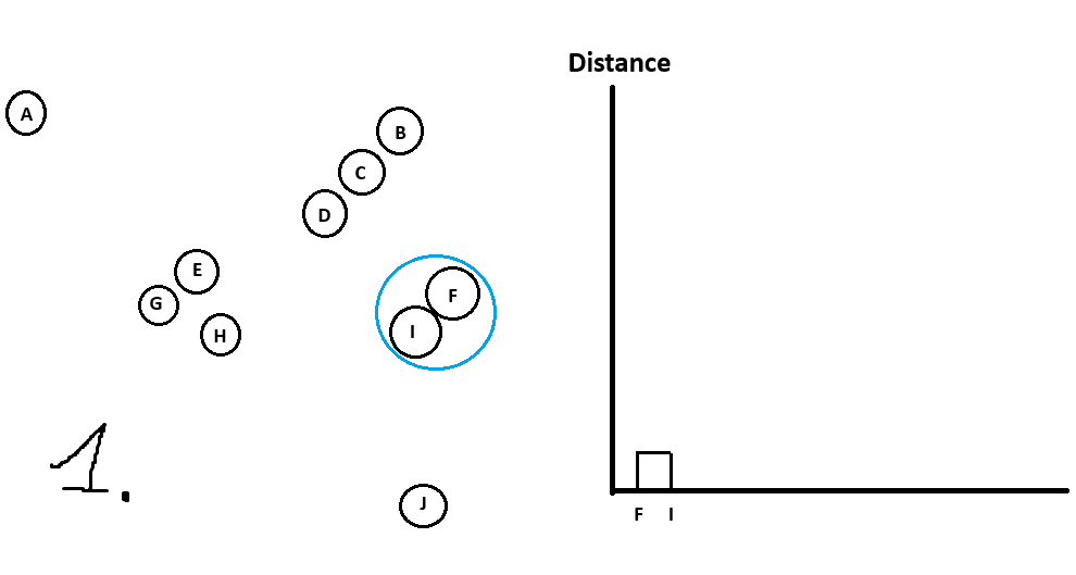
See which data point is closest to data point #1.
See which data point is closest to data point #2.
…
See which data point is closest to data point #n.
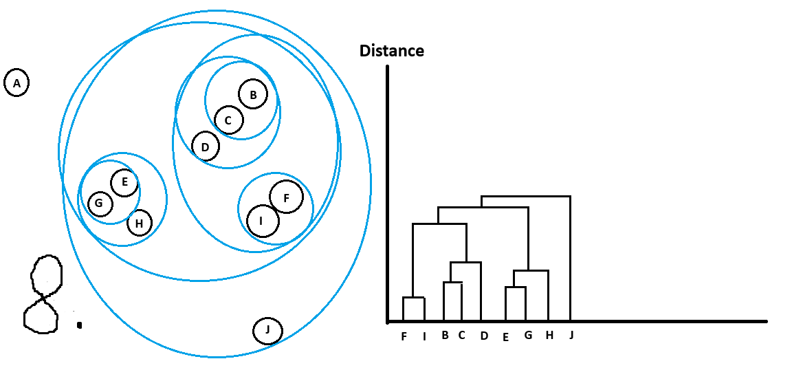
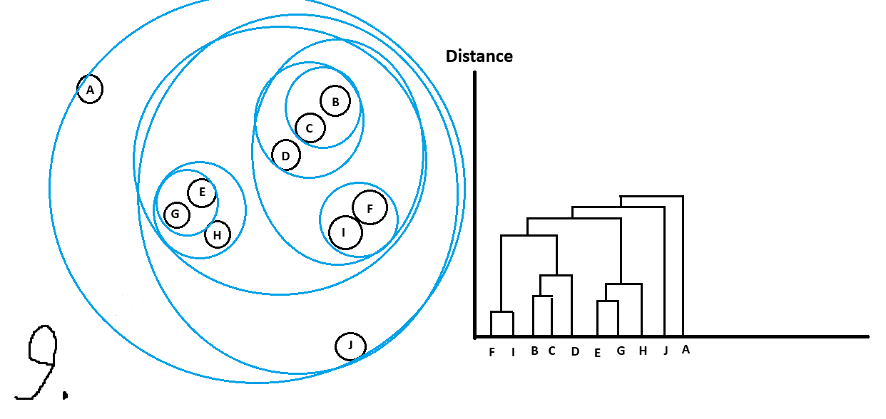
Whatever 2 points are closest to each other will form cluster #1.Repeat step 1 but treat clusters like their own data points (can use the mean of the cluster) until you are left with all data points in 1 big cluster.
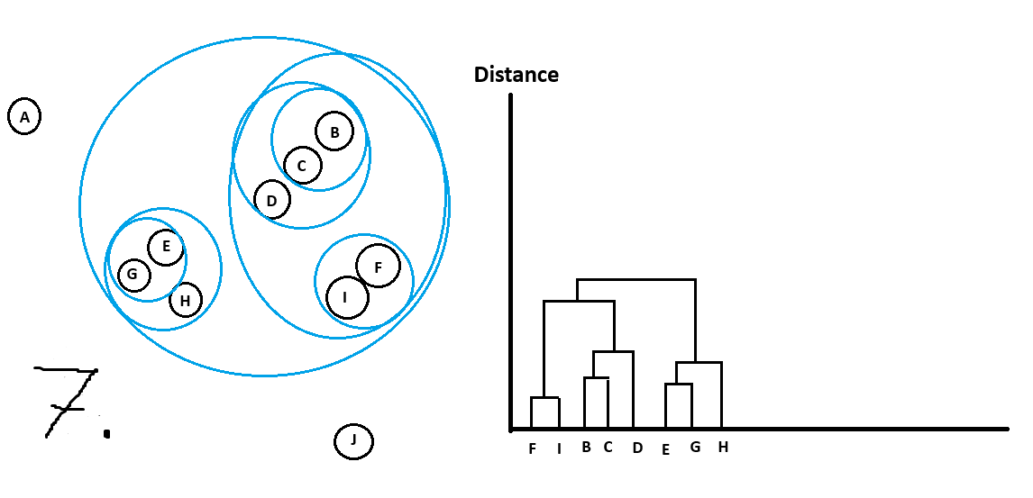
Whenever we form a new cluster we add it to the dendrogram.
Let’s walk through an example:
And with that we are done!
Can see all the clusters with their sub-clusters.
Just like with OPTICS there are different ways to get main clusters from the dendrogram.
For example I could do the following cutoff in distance and get the following clusters
which we would have picked intuitively too!
Max-Min-Distance Clustering
This clustering technique is our first graph-based one.
I’ve actually written a little thread on it recently over on my twitter, you can check it out here:
https://twitter.com/Vertox_DF/status/1721251065843065275
Dimensionality Reduction
Let’s say you have some data that is 1000 dimensional.
For example, an asset and its time series.
While clustering on this would be possible since distance metrics like the Euclidian distance work even for 1000D data there are some reasons as to why you should reduce the dimension of your data.
Curse of Dimensionality
As the number of dimensions in your dataset increases the amount of data you need increases exponentially and your data becomes more and more sparse.
This makes it harder to find clusters.Computational Efficiency
This one is straightforward, the more dimensions you have the more computing power you will need to calculate the distances.
Noise
High dimensional data is gonna be very noisy, with dimensionality reduction we try to only extract the most important information.
Visualization
Hard to visualize higher than 2D or 3D data in a nice way.
There are a lot of different dimensionality reduction techniques.
The most common ones are:
PCA
t-SNE
Isomap
LDA
Autoencoder
Features
etc.
For asset returns specifically, you can also use features like average return and volatility and cluster based on those 2 data points instead of the entire time series.
Final Remarks
That was a pretty long post!
Didn’t want to get into the full detail of dimensionality reduction in this one as that’s a whole nother rabbit hole. If you guys do want to see a detailed article on that let me know!


