Common Risk Metrics (PyNL Part 1)

The first part of developing a quant python library

Sep 30, 2024

One of the first things a new firm does is developing some research tools. You wanna make sure you can do research quickly and efficiently and be able to iterate as quickly as possible.

So we are gonna be developing a python library full of research tools like:

Risk Metrics
Useful Plots
Backtesters
Data Gatherers (Scrapers etc.)
Data Processors
etc.

I will also be using the library to do a lot of the research for the substack!

Table of Content

Sharpe Ratio
Sortino Ratio
Maximum Drawdown
Calmar Ratio
Beta
Treynor Ratio
Information Ratio
CDF of Returns Plot
Omega Ratio
Value at Risk (VaR)
Conditional Value at Risk (CVaR)
Drawdown Plot
Final Remarks

Sharpe Ratio

Let’s start off simple with the most important metric: The sharpe ratio.

It’s defined the following way:

With:

R_p = Portfolio Returns
R_f = Risk-free Return
sigma_p = Standard Deviation of Portfolio Returns

Before we code the function we are gonna import a few numpy functions:

from numpy import array, mean, std, var, cov, sqrt, maximum, unique, cumsum, argmax

And now we can code up the calculation for sharpe:

#equity_arr = array of returns
#T = Trading window length in years
#risk_free_rate = Risk-free return pre year
def sharpe_ratio(equity_arr, T, risk_free_rate = 0):
    equity_arr = array(equity_arr)

    returns = (equity_arr[1:] - equity_arr[:-1]) / equity_arr[:-1]

    return_mean = mean(returns)
    return_std = std(returns)

    trades_per_year = len(returns) / T

    yearly_return = return_mean * trades_per_year
    yearly_excess_return = yearly_return - risk_free_rate

    annualized_std = sqrt(trades_per_year) * return_std

    sharpe_ratio = yearly_excess_return / annualized_std

    return sharpe_ratio

That looks a little more complicated than what we have in the formula, let me explain.

Most important is normalizing our sharpe in some way and what’s done in practice is annualizing it.

So let’s say we have a strategy that trades on the daily timeframe and is invested in the market 20% of the time. 20% of a year is 73 days so we need to multiply our average daily return by 73 to get our average yearly return.

To get our std of yearly returns we do sqrt(73) * std(daily returns) since volatility roughly follows:

Where sigma is the volatility for 1 measure of time and sigma_T is the volatility for T measures of time.

Sortino Ratio

Instead of using the volatility of all returns we use the volatility of just the negative returns.

The idea is that we shouldn’t punish strong volatility if the returns are still positive.

The change to the code is very simple, we just have negative_returns = returns[returns < 0] and use the std of that.

#equity_arr = array of returns
#T = Trading window length in years
#risk_free_rate = Risk-free return pre year
def sortino_ratio(equity_arr, T, risk_free_rate = 0):
    equity_arr = array(equity_arr)

    returns = (equity_arr[1:] - equity_arr[:-1]) / equity_arr[:-1]

    return_mean = mean(returns)

    neg_returns = returns[returns < 0]
    neg_return_std = std(neg_returns)

    trades_per_year = len(returns) / T

    yearly_return = return_mean * trades_per_year
    yearly_excess_return = yearly_return - risk_free_rate

    annualized_std = sqrt(trades_per_year) * neg_return_std

    sortino_ratio = yearly_excess_return / annualized_std

    return sortino_ratio

Maximum Drawdown

You calculate the drawdown by first calculating the peak equity timeseries which would look something like this:

Your maximum drawdown is then your smallest percent change from peak[t] to equity[t] (Or equity[t] - peak[t] if you want the maximum absolute drawdown).

#equity_arr = array of equity
def max_drawdown(equity_arr, absolute=False):
    equity_arr = array(equity_arr)

    peak = maximum.accumulate(equity_arr)

    if not absolute:
        drawdown = (equity_arr - peak) / peak
    else:
        drawdown = equity_arr - peak

    max_drawdown = min(drawdown)

    return max_drawdown

we do min(drawdown) since drawdown is a negative number.

Calmar Ratio

The calmar ratio is defined as yearly excess return / maximum drawdown.

The code to calculate it is:

#equity_arr = array of equity
#T = Trading window length in years
#risk_free_rate = Risk-free return pre year
def calmar_ratio(equity_arr, T, risk_free_rate = 0):
    equity_arr = array(equity_arr)
    returns = (equity_arr[1:] - equity_arr[:-1]) / equity_arr[:-1]

    return_mean = mean(returns)

    trades_per_year = len(returns) / T

    yearly_return = return_mean * trades_per_year
    yearly_excess_return = yearly_return - risk_free_rate

    max_dd = max_drawdown(equity_arr)

    calmar_ratio = - yearly_excess_return / max_dd

    return calmar_ratio

Beta

Beta measures the volatility of something compared to something else (usually an index).

You could have the beta of TSLA 0.00%↑ compared to SPY 0.00%↑ for example.

It’s defined as:

where R_p is our portfolio returns and R_b our benchmark returns.

The code to calculate this is pretty simple:

#equity_arr = array of equity
#benchmark_equity_arr = array of equity of benchmark
def beta(equity_arr, benchmark_equity_arr):
    equity_arr = array(equity_arr)
    benchmark_equity_arr = array(benchmark_equity_arr)

    returns = (equity_arr[1:] - equity_arr[:-1]) / equity_arr[:-1]
    benchmark_returns = (benchmark_equity_arr[1:] - benchmark_equity_arr[:-1]) / benchmark_equity_arr[:-1]

    beta = cov(returns, benchmark_returns)[0, 1] / var(benchmark_returns)

    return beta

Treynor Ratio

The treynor ratio is defined as yearly excess return / beta so the code is:

#equity_arr = array of equity
#benchmark_equity_arr = array of equity of benchmark
#T = Trading window length in years
#risk_free_rate = Risk-free return pre year
def treynor_ratio(equity_arr, benchmark_equity_arr, T, risk_free_rate = 0):
    equity_arr = array(equity_arr)
    returns = (equity_arr[1:] - equity_arr[:-1]) / equity_arr[:-1]

    return_mean = mean(returns)

    trades_per_year = len(returns) / T

    yearly_return = return_mean * trades_per_year
    yearly_excess_return = yearly_return - risk_free_rate

    beta = beta(equity_arr, benchmark_equity_arr)

    treynor_ratio = yearly_excess_return / beta

    return treynor_ratio

Information Ratio

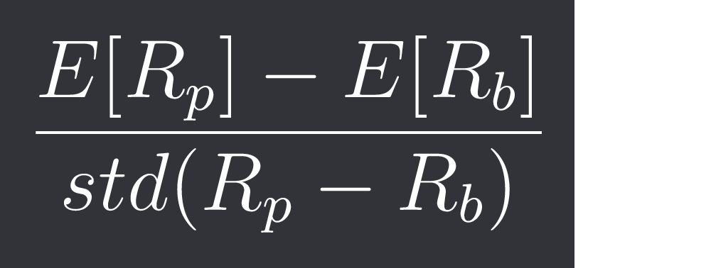
This one is a little more interesting. We look at the spread between our portfolio and the benchmark.

With that the Information Ratio is defined as:

The code for this is:

#equity_arr = array of equity
#benchmark_equity_arr = array of equity of benchmark
#T = Trading window length in years
def information_ratio(equity_arr, benchmark_equity_arr, T):
    equity_arr = array(equity_arr)
    benchmark_equity_arr = array(benchmark_equity_arr)

    returns = (equity_arr[1:] - equity_arr[:-1]) / equity_arr[:-1]
    benchmark_returns = (benchmark_equity_arr[1:] - benchmark_equity_arr[:-1]) / benchmark_equity_arr[:-1]

    spread_returns = returns - benchmark_returns

    return_mean = mean(returns)
    benchmark_return_mean = mean(benchmark_returns)

    trades_per_year = len(returns) / T
    benchmark_trades_per_year = len(benchmark_returns) / T

    yearly_return = return_mean * trades_per_year
    benchmark_yearly_return = benchmark_return_mean * benchmark_trades_per_year

    spread_std = std(spread_returns)

    information_ratio = (yearly_return - benchmark_yearly_return) / spread_std

    return information_ratio

CDF of Returns Plot

Before we can look at the omega ratio we need to first look at the cumulative density function of our portfolio returns defined as:

So for r = 0.05 F_R(r) would be the probability of a random return of our portfolio being smaller than or equal to r.

Note: I always talk about a “portfolio” but it can really be whatever you want.

Calculating this cumulative probability is pretty easy:

equity_arr = array(equity_arr)
returns = (equity_arr[1:] - equity_arr[:-1]) / equity_arr[:-1]

unique_returns, counts = unique(returns, return_counts=True)
cum_probs = cumsum(counts) / len(returns)

Note that we need a sorted array of returns! unique() luckily does that for us already.

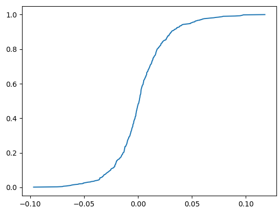
If we plot unique_returns vs cum_probs for some daily BTC data we get:

Now let’s make this plot a little better looking:

def plot_return_cdf(equity_arr):
    equity_arr = array(equity_arr)
    returns = (equity_arr[1:] - equity_arr[:-1]) / equity_arr[:-1]

    unique_returns, counts = unique(returns, return_counts=True)
    cum_probs = cumsum(counts) / len(returns)

    # Plot the CDF
    plt.figure(figsize=(8, 6))
    plt.plot(unique_returns, cum_probs, color='grey')
    plt.axvline(0, color='grey', linestyle='--')
    plt.fill_between(unique_returns, cum_probs, where=unique_returns < 0, color='red', alpha=0.5)
    plt.fill_between(unique_returns, cum_probs, 1, where=unique_returns >= 0, color='green', alpha=0.5)
    plt.xlabel('Returns')
    plt.ylabel('Cumulative Probability')
    plt.title('Cumulative Distribution of Returns')
    plt.grid(True)

    plt.tight_layout()
    plt.show()

Looks pretty good! We need this plot to understand the omega ratio.

Omega Ratio

The omega ratio is defined as the green area divided by the red area.

Calculating those is pretty easy, imagine our CDF looked like this:

Calculating the area under the curve would then just mean summing up the area of a bunch of rectangles and triangles (1/2 of a rectangle).

Note: once we calculate the area under the curve for the negative and positive returns we need to subtract the area under the positive returns from the largest unique return to get the green area in the CDF plot (area ABOVE the curve).

Here is the code that does all that for us and returns the omega ratio:

#equity_arr = array of equity
def omega_ratio(equity_arr):
    equity_arr = array(equity_arr)
    returns = (equity_arr[1:] - equity_arr[:-1]) / equity_arr[:-1]

    unique_returns, counts = unique(returns, return_counts=True)
    cum_probs = cumsum(counts) / len(returns)

    red_area = 0
    green_area = 0
    for i in range(len(unique_returns)-1):
        if unique_returns[i] < 0:
            if unique_returns[i+1] <= 0:
                width = unique_returns[i+1]-unique_returns[i]
                red_area += cum_probs[i]*width + ((cum_probs[i+1] - cum_probs[i])*width) / 2
            else:
                width = -unique_returns[i]
                slope = (cum_probs[i+1]-cum_probs[i])/(unique_returns[i+1]-unique_returns[i])

                zero_height = cum_probs[i] + width*slope

                red_area += cum_probs[i]*width + ((zero_height - cum_probs[i])*width) / 2
                green_area += zero_height*unique_returns[i+1] + ((cum_probs[i+1] - zero_height)*unique_returns[i+1]) / 2
        else:
            width = unique_returns[i+1]-unique_returns[i]
            green_area += cum_probs[i]*width + ((cum_probs[i+1] - cum_probs[i])*width)/2

    green_area = unique_returns[-1] - green_area

    omega_ratio = green_area / red_area

    return omega_ratio

Value at Risk (VaR)

Given a confidence parameter alpha, VaR is defined as the biggest lost we expect to see with 1-alpha % certainty. So for example with an alpha of 5% we could say that we won’t face a loss larger than x% with 95% certainty.

We can read that value directly from the CDF plot!

Visually we can tell that with 90% certainty our loss will not be bigger than -2.5%.

Here is the code to get that value:

#equity_arr = array of equity
def VaR(equity_arr, alpha=0.05):
    equity_arr = array(equity_arr)
    returns = (equity_arr[1:] - equity_arr[:-1]) / equity_arr[:-1]

    unique_returns, counts = unique(returns, return_counts=True)
    cum_probs = cumsum(counts) / len(returns)

    idx = argmax(cum_probs >= alpha)
    
    if cum_probs[idx] >= alpha:
        return unique_returns[idx]
        
    return None

Plugging our array and 0.1 into the function we get -2.54% so we were super close!

Conditional Value at Risk (CVaR)

One problem of VaR is that it doesn’t tell you much about how much risk you potentially have (tail risk).

CVaR tries to solve it by giving you the average return for returns smaller than the VaR.

We can simply just use mean().

#equity_arr = array of equity
def CVaR(equity_arr, alpha=0.05):
    equity_arr = array(equity_arr)
    returns = (equity_arr[1:] - equity_arr[:-1]) / equity_arr[:-1]

    unique_returns, counts = unique(returns, return_counts=True)
    cum_probs = cumsum(counts) / len(returns)

    idx = argmax(cum_probs >= alpha)
    
    if cum_probs[idx] >= alpha:
        worse_returns = returns[returns <= unique_returns[idx]] 

        return mean(worse_returns)
        
    return None

Drawdown Plot

We’ve already calculated the drawdown array for our equity in the maximum drawdown section.

Let’s plot that and price and also make the plot more pretty by doing things like making the price plot green where it’s not in a drawdown and red where it is in a drawdown:

#equity_arr = array of equity
#absolute = If equity is given in dollar-terms or relative performance
def plot_drawdown(equity_arr, absolute=False):
    drawdown_arr = []
    peak_arr = []
    peak = equity_arr[0]

    up_peaks = []
    up_indexes = []

    down_peaks = []
    down_indexes = []

    peaks_section = [equity_arr[0]]
    indexes_section = [0]
    direction = 0


    if equity_arr[1] >= equity_arr[0]:
        direction = 1   
    else:
        direction = -1

    for idx, cur_equity in enumerate(equity_arr):
        old_peak = peak

        peak = max(peak, cur_equity)
        peak_arr.append(peak)

        if idx > 0:
            if cur_equity >= old_peak and direction == 1:
                peaks_section.append(peak)
                indexes_section.append(idx)
            elif cur_equity > old_peak and direction == -1:
                down_peaks.append(peaks_section)
                down_indexes.append(indexes_section)

                peaks_section = []
                indexes_section = []

                peaks_section.append(old_peak)
                indexes_section.append(idx-1)
                peaks_section.append(peak)
                indexes_section.append(idx)

                direction = 1
            elif cur_equity <= old_peak and direction == -1:
                peaks_section.append(peak)
                indexes_section.append(idx)
            elif cur_equity < old_peak and direction == 1:
                up_peaks.append(peaks_section)
                up_indexes.append(indexes_section)

                peaks_section = []
                indexes_section = []

                peaks_section.append(old_peak)
                indexes_section.append(idx-1)
                peaks_section.append(peak)
                indexes_section.append(idx)

                direction = -1

        if not absolute:
            drawdown = (cur_equity - peak_arr[-1]) / peak_arr[-1]  
        else:
            drawdown = cur_equity - peak_arr[-1]

        drawdown_arr.append(drawdown) 

    if direction == 1:
        up_peaks.append(peaks_section)
        up_indexes.append(indexes_section)
    else:
        down_peaks.append(peaks_section)
        down_indexes.append(indexes_section)


    fig, (ax1, ax2) = plt.subplots(2, 1, figsize=(10, 8))

    ax1.plot(equity_arr, label="Equity", color='tab:blue')

    for i in range(len(up_peaks)):
        ax1.plot(up_indexes[i], up_peaks[i], color='green')
    for i in range(len(down_peaks)):
        ax1.plot(down_indexes[i], down_peaks[i], color='red')
    
    ax1.fill_between(range(len(equity_arr)), peak_arr, equity_arr, color='blue', alpha=0.3)
    ax1.set_title("Equity over Time")
    ax1.set_xlabel("Time")
    ax1.set_ylabel("Equity")
    ax1.grid(True)
    ax1.legend()

    ax2.plot(drawdown_arr, label="Drawdown", color='tab:red')
    ax2.axhline(0, linestyle='--', color='grey')
    ax2.fill_between(range(len(drawdown_arr)), drawdown_arr, 0, color='red', alpha=0.3)
    ax2.set_title("Drawdown over Time")
    ax2.set_xlabel("Time")
    ax2.set_ylabel("Drawdown")
    ax2.grid(True)
    ax2.legend()

    plt.tight_layout()
    plt.show()

Here is what that looks like for daily $BTC data:

Final Remarks

That’s it for the first dev post of the PyNL library!
If you have any recommendations or features you wish implemented feel free to comment that down below!

Note: Dev posts will not interfere with the frequency of the usual posts, those will still appear once a week and in addition you will get PyNL posts!

VertoxQuant

Discussion about this post