Forecasting Runescape Prices

A fun project using our quant skills

Feb 07, 2025

It’s not a secret that OSRS is one of the favorite games and that I’ve spent a lot of time trading on the Grand Exchange.

One thing I’ve noticed while trading there: Prices are very easy to predict.
This makes sense, you wouldn’t expect an in-game market to be super efficient.

With OSRS I noticed a lot of seasonalities (I also noticed this in other video game marketplaces like the steam marketplace) and momentum.

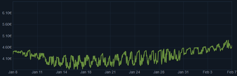
Median sale price of Spektrum Cases in CS2

Table of Content

Runescape API
Exploratory Data Analysis
Price Prediction Model
Final Remarks

Runescape API

There are many APIs available to get historical grand exchange price and volume data.
We are gonna be using the following one:
https://api.weirdgloop.org/

We need to call /exchange/history/{game}/{filter} where we will set:

game: “osrs”
filter: “all?id={id}”

Every item in the game has a unique ID that you can find on the following site:
https://www.osrsbox.com/tools/item-search/

One important and heavily traded type of item in the game are runes. The following runes exist with their respective IDs:

Free 2 Play Runes:

Fire: 554
Water: 555
Air: 556
Earth: 557
Mind: 558
Body: 559
Death: 560
Nature: 561
Chaos: 562
Law: 563
Cosmic: 564

Member Runes:

Blood: 565
Soul: 566
Astral: 9075
Wrath: 21880
Sunfire: 28929

Combination Runes:

Steam: 4694
Mist: 4695
Dust: 4696
Smoke: 4697
Mud: 4698
Lava: 4699

Let’s write some python code to get the historical prices for all those items:

import pandas as pd
import numpy as np
import matplotlib.pyplot as plt
import requests
import json
import traces
from datetime import datetime, timedelta

items = {}
for item in item_ids.keys():
    request = requests.get(f"https://api.weirdgloop.org/exchange/history/osrs/all?id={item_ids[item]}")

    data = request.json()[str(item_ids[item])]

    timestamps = []
    prices = []
    volumes = []

    for datapoint in data:
        timestamps.append(datapoint["timestamp"])
        prices.append(datapoint["price"])
        volumes.append(datapoint["volume"])

    items[item] = pd.DataFrame({"Price": prices, "Volume": volumes}, index=timestamps)
    items[item].index = pd.to_datetime(items[item].index*1000000)

Here is one of the runes:

As you can see the data goes very far back although we have no volume for those early data points. Also as you can see they grab the data at pretty random times of day for those recent data points that aren’t equally spaced but we need equally spaced data for our data analysis and model building so we will use linear interpolation using the traces library to resample our data at daily frequencies.

Our final code for getting price data is:

item_ids = {
    "Fire": 554,
    "Water": 555,
    "Air": 556,
    "Earth": 557,
    "Mind": 558,
    "Body": 559,
    "Death": 560,
    "Nature": 561,
    "Chaos": 562,
    "Law": 563,
    "Cosmic": 564,
    "Blood": 565,
    "Soul": 566,
    "Astral": 9075,
    "Wrath": 21880,
    "Sunfire": 28929,
    "Steam": 4694,
    "Mist": 4695,
    "Dust": 4696,
    "Smoke": 4697,
    "Mud": 4698,
    "Lava": 4699
}

items_list = item_ids.keys()

items = {}
for item in items_list:
    request = requests.get(f"https://api.weirdgloop.org/exchange/history/osrs/all?id={item_ids[item]}")

    data = request.json()[str(item_ids[item])]

    timestamps = []
    prices = []
    volumes = []

    for datapoint in data:
        timestamps.append(datapoint["timestamp"])
        prices.append(datapoint["price"])
        volumes.append(datapoint["volume"])

    items[item] = pd.DataFrame({"Price": prices, "Volume": volumes}, index=timestamps)
    items[item].index = pd.to_datetime(items[item].index*1000000)

    ts_price = traces.TimeSeries(dict(zip(items[item].index, items[item]["Price"])))
    ts_volume = traces.TimeSeries(dict(zip(items[item].index, items[item]["Volume"])))

    sampled_price = ts_price.sample(sampling_period=timedelta(days=1), interpolate='linear')
    sampled_volume = ts_volume.sample(sampling_period=timedelta(days=1), interpolate='linear')

    items[item] = pd.DataFrame.from_dict(dict(sampled_price), orient="index", columns=["Price"])
    items[item]["Volume"] = pd.DataFrame.from_dict(dict(sampled_volume), orient="index", columns=["Volume"])

    items[item].index = pd.to_datetime(items[item].index)

Exploratory Data Analysis

Let’s plot our data:

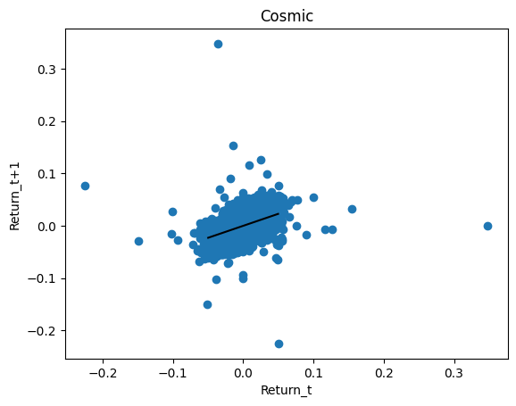
The cosmic rune looks particularly interesting, let’s plot that one separately:

Let’s get the returns of those items:

for item in items_list:
    items[item]["Return"] = items[item]["Price"].pct_change(1)
    items[item].dropna(inplace=True)

Those are some really nicely behaving returns, let’s look at the distribution:

The reason you see no really small returns is because of the ticksize of 1 (150/149 - 1 would be a 0.67% return for example).

I mainly suspect 2 effects that will be very useful in predicting returns: seasonality and autocorrelation of returns.

There are a lot of runes with a very low price or with very low trading activities so we are gonna get rid of those in our analysis:

Lava
Dust
Sunfire
Body
Mind
Earth
Air
Water
Fire

Price Prediction Model

Autocorrelation of returns:

This is simpler to test so we are gonna start with that.
Let’s plot the partial autocorrealtion function of returns for each rune:

from statsmodels.graphics.tsaplots import plot_pacf

for item in items_list:
    plot_pacf(items[item]["Return"], zero=False)
    plt.title(f"{item} PACF of return")
    plt.show()

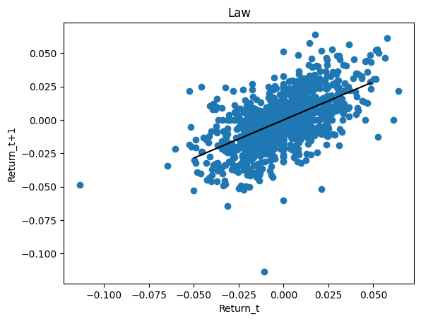
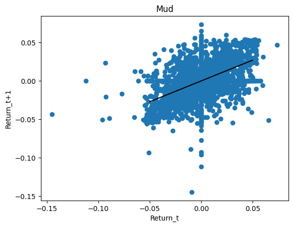
Like expected our runes show strong positive autocorrelation in returns so let’s regress without intercept returns against next day returns excluding zeros outliers:

import statsmodels.api as sm

slopes = {}
for item in items_list:
    ret_t = items[item]["Return"].iloc[:-1][(np.array(items[item]["Return"].iloc[:-1]) != 0) & (np.array(items[item]["Return"].iloc[1:]) != 0) & (abs(np.array(items[item]["Return"].iloc[:-1])) <= 0.05)].values
    ret_t1 = items[item]["Return"].iloc[1:][(np.array(items[item]["Return"].iloc[:-1]) != 0) & (np.array(items[item]["Return"].iloc[1:]) != 0) & (abs(np.array(items[item]["Return"].iloc[:-1])) <= 0.05)].values

    model = sm.OLS(ret_t, ret_t1)
    results = model.fit()

    slope = results.params[0]

    slopes[item] = slope

    plt.scatter(items[item]["Return"].iloc[:-1], items[item]["Return"].iloc[1:])
    plt.plot([min(ret_t), max(ret_t)], slope*np.array([min(ret_t), max(ret_t)]), color="black")
    plt.title(item)
    plt.xlabel("Return_t")
    plt.ylabel("Return_t+1")
    plt.show()

Let’s see how well trading this would have performed on Nature runes without any fees and assuming we trade at the given price instantly etc. etc:

equity = [1]
for i in range(len(items["Nature"])-1):
    prediction = slopes["Nature"]*items["Nature"]["Return"].iloc[i]
    
    if prediction > 0:
        equity.append(equity[-1] * (1 + items["Nature"]["Return"].iloc[i+1]))
    else:
        equity.append(equity[-1])

Well that’s quite a return. Unfortunately we have a 1% fee when trading on OSRS (as of late 2021 but we are just gonna assume it for the entire duration for simplicity) so let’s include that:

equity = [1]

position = 0
for i in range(len(items["Nature"])-1):
    fees = 0
    prediction = slopes["Nature"]*items["Nature"]["Return"].iloc[i]
    
    if prediction > 0.01:
        position = 1
        
    if position == 1 and prediction < 0:
        position = 0
        fees = 0.01

    equity.append(equity[-1] * (1 + position*items["Nature"]["Return"].iloc[i+1] - fees))

Seasonality:

The seasonality comes from when players are active. Prices go up when there are fewer people online and go down when more players are online. I therefore expect a seasonality in the time of day (although we are working with daily data so we will ignore that) and a seasonality in the day of week.

for item in items_list:
    items[item]["DayOfWeek"] = items[item].index.weekday

for item in items_list:
    mean_volumes = []
    mean_returns = []
    for day in range(7):
        mean_volumes.append(np.mean(np.array(items["Chaos"]["Volume"].iloc[1:])[items["Chaos"]["DayOfWeek"].iloc[:-1] == day]))
        mean_returns.append(np.mean(np.array(items["Chaos"]["Return"].iloc[1:])[items["Chaos"]["DayOfWeek"].iloc[:-1] == day]))

    seasonality[item] = mean_returns

    plt.bar(range(7), mean_volumes)
    plt.xlabel("Day of week")
    plt.ylabel("Mean(Return)")
    plt.title(item)
    plt.show()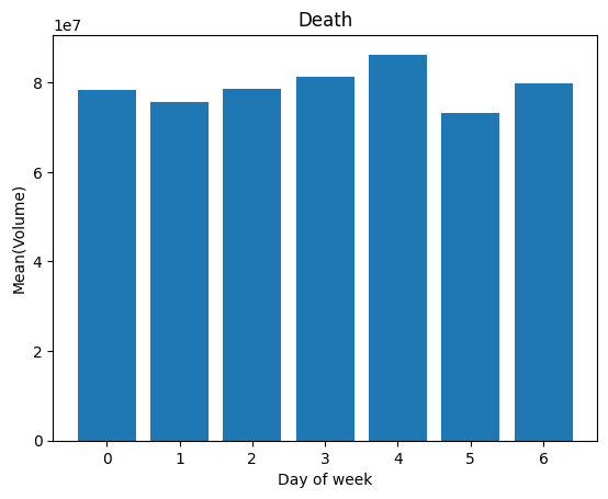

The returns also show strong similarity:

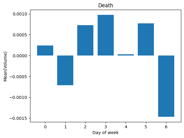
After running some backtests we don’t seem to be getting any good results and it mostly looks like random walks so I’m not gonna include them.

Note: In reality our trading results probably wouldn’t have been *as* good because we tested on our training set but either way osrs prices are clearly very predictable and tradable.

Final Remarks

I hope you guys enjoyed this fun little side project. If you are more serious about this you can of course expand on it and work on it even more (If you do you can let me know cuz I’ll be interested in seeing some interesting OSRS data!).
This articles purpose was mainly to show you that you can use your quant skills outside of financial markets.

VertoxQuant

Discussion about this post