How Market Making Models work

and what they have in common with inverted pendulums

In this article, we are gonna be covering how market making models work mathematically and how you can design your own market making model!

Before we get into market making, we are first gonna figure out the mathematics behind a more general idea… balancing a pendulum upside down.

Pendulum on a Cart

Consider my awesome drawing of a pendulum attached to a car:

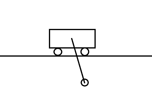
We are able to apply a force (u) to the car (positive to move it right and negative to move it left). Are we able to balance the pendulum at the top just by doing that?
Yes, we are! Ever balanced a broom on your hand as a kid? Same principle.

Great, just how on earth do we do this, though?

First, we need to figure out the dynamics of our system. Let’s say we are able to measure a few things:

• x: The position of the car

• x’: The speed of the car

• theta: The angle of the pendulum

• theta’: The rate of change of the angle.

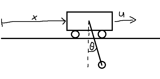
Those 4 things make up a “state” of our system.

\(\bar{x} = \begin{bmatrix} x \\ \dot{x} \\ \theta \\ \dot{\theta} \end{bmatrix}\)

I’m not gonna bore you with the derivation of the physical system here, I’m not a physicist. Just trust me that the physical system here is:

\(\begin{align} \ddot{\theta} &= -\frac{L^2m^2\dot{\theta}^2 \sin(2\theta) + 2Lgm(M+m)\sin\theta + 2Lmu(t)\cos\theta + 2\delta(M+m)\dot{\theta}}{2L^2m(M+m\sin^2 \theta)} \\ \ddot{x} &= \frac{L^2m\dot{\theta}^2\sin\theta + \frac{1}{2}Lgm\sin(2\theta) + Lu(t) + c\dot{\theta}\cos\theta}{L(M+m\sin^2\theta)} \end{align}\)

There are a ton of symbols here… let’s make sense of them:

• L: Length of the pendulum

• M: Mass of the car

• m: Mass of the pendulum

• g: Gravitational constant

• delta: Damping torque

Let’s simulate this with just a constant force:

import numpy as np
import matplotlib.pyplot as plt
from matplotlib.animation import FuncAnimation
import matplotlib.animation as animation
from scipy.integrate import solve_ivp
from scipy.linalg import solve_continuous_are

duration=10
fps = 60

# Parameters
M = 2.0      # cart mass
m = 1      # pendulum mass
L = 2.0      # pendulum length
delta = 0.001 # Pendulum drag


g = 9.81

theta0 = np.pi - 0.75
theta_dot0 = 0
x0 = 0
x_dot0 = 0


# Control input (force on cart)
def u():
    return 0.5
    

# ODE system
def dynamics(t, y):
    x, x_dot, theta, theta_dot = y

    # --- with viscous pivot damping c = delta ---
    denom = (M + m*np.sin(theta)**2)
    theta_ddot = -(
        (L**2 * m**2 * theta_dot**2 * np.sin(2*theta))
        + 2*L*g*m*(M+m)*np.sin(theta)
        + 2*L*m*u()*np.cos(theta) 
        + 2*delta*(M+m)*theta_dot
    ) / (2 * L**2 * m * denom)

    x_ddot = (
        (L**2 * m * theta_dot**2 * np.sin(theta))
        + 0.5*L*g*m*np.sin(2*theta)
        + L*u()
        + delta*theta_dot*np.cos(theta)
    ) / (L * denom)

    return [x_dot, x_ddot, theta_dot, theta_ddot]

t_eval = np.linspace(0, duration, int(duration*fps/2))
sol = solve_ivp(dynamics, [0, duration], [x0, x_dot0, theta0, theta_dot0], t_eval=t_eval)

# Extract solution
x, theta = sol.y[0], sol.y[2]

# Convert to x, y coordinates
pendulum_x = x + L * np.sin(theta)
pendulum_y = -L * np.cos(theta)

# --- Animation setup ---
fig, ax = plt.subplots(figsize=(8, 5))
ax.set_xlim(np.min(x) - L - 0.5, np.max(x) + L + 0.5)
ax.set_ylim(-1.5*L, 1.5*L)
ax.set_aspect(’equal’)
ax.set_xlabel(”x position (m)”)
ax.set_title(”Pendulum on a Cart Simulation”)

# Elements to animate
track, = ax.plot([], [], ‘k-’, lw=2)
cart, = ax.plot([], [], ‘s’, color=’tab:blue’, markersize=20)
rod, = ax.plot([], [], ‘o-’, color=’tab:orange’, lw=2, markersize=10)
time_text = ax.text(0.02, 0.9, ‘’, transform=ax.transAxes)

# --- Initialization ---
def init():
    track.set_data([], [])
    cart.set_data([], [])
    rod.set_data([], [])
    time_text.set_text(’‘)
    return track, cart, rod, time_text

# --- Animation update function ---
def update(i):
    cart_x = x[i]
    cart_y = 0.0

    # Pendulum line endpoints
    rod_x = [cart_x, pendulum_x[i]]
    rod_y = [cart_y, pendulum_y[i]]

    # Track line
    track.set_data([np.min(x) - L, np.max(x) + L], [0, 0])

    cart.set_data([cart_x], [cart_y])
    rod.set_data(rod_x, rod_y)
    time_text.set_text(f”t = {sol.t[i]:.2f} s”)
    return track, cart, rod, time_text

# --- Create animation ---
ani = FuncAnimation(
    fig, update, frames=len(t_eval),
    init_func=init, interval=1/fps, blit=True
)

import imageio_ffmpeg, matplotlib
matplotlib.rcParams[’animation.ffmpeg_path’] = imageio_ffmpeg.get_ffmpeg_exe()

writer = animation.FFMpegWriter(fps=fps, bitrate=9000)  # ~9 Mbps
ani.save(”inverted_pendulum.mp4”, writer=writer, dpi=120)

plt.show()

Before we continue with the pendulum example, we need to understand some theory first.

Linear System of ODEs

Consider the following linear system of ODEs:

\(\dot{x} = Ax\)

The solution to this is given by

\(x(t) = e^{At}x(0)\)

e to the power of a matrix? What the hell? Actually, it’s pretty simple if we look at the Taylor series of the exponential:

\(e^{At} = \sum_{n=0}^{\infty} \frac{(At)^n}{n!} = I + \sum_{n=1}^{\infty} \frac{A^nt^n}{n!}\)

Don’t worry, you won’t actually have to evaluate this.

Instead, we can do something really cool called diagonalization, where we rewrite A as follows:

\(A = TDT^{-1}\)

Where D is a diagonal matrix made up of eigenvalues of A, and T is a matrix made up of eigenvectors of A. For more details on when exactly a matrix is and isn’t diagonalizable, check out the Wikipedia page: https://en.wikipedia.org/wiki/Diagonalizable_matrix

As a rule of thumb, most normal matrices that you work with are probably diagonalizable.

What happens if we take A to the power of two now?

\(A^2 = TDT^{-1}TDT^{-1} = TDDT^{-1} = TD^2T^{-1}\)

Oh, that’s neat, the power moved into the diagonal matrix.
In fact, for any n, we have:

\(A^n = TD^nT^{-1}\)

Plugging this into the definition of e^{At}, we also see pretty easily that:

\(e^{At} = Te^{Dt}T^{-1}\)

Cool… so instead of having to calculate e^{At}, we now have to diagonalize A and STILL calculate a matrix exponential e^{Dt}. What’s the point?

The point is that calculating the exponential of a diagonal matrix is incredibly easy.
The solution is:

\(e^{Dt} = \begin{bmatrix} e^{\lambda_1t} & & \\ & \ddots & \\ & & e^{\lambda_nt} \end{bmatrix}\)

Where lambda_i*t is the ith diagonal entry of Dt, and those lambdas are the eigenvalues of A. So we just have to diagonalize and then take exponents of SCALARS, which is super easy.

Plugging this back into the solution of our linear system of ODEs:

\(x(t) = Te^{Dt}T^{-1}x(0)\)

What can we say about the stability of this solution? Does it blow up to infinity? Does it converge towards 0? Does it oscillate? The solution lies inside our matrix e^{Dt}!

Eigenvalues are complex numbers:

\(\lambda = a\pm ib\)

From complex analysis, we have that each of our diagonal entries of e^{Dt} is of the form:

\(e^{\pm \lambda t} = e^{a t}[cos(bt) \pm i sin(bt)]\)

The part inside the brackets always has an amplitude of 1, and so we don’t have to worry about it. The e^{at}, however, will blow up for a > 0 and converge to 0 for a < 0.

a is the real part of our eigenvalue, so we come to the final conclusion:

Our system’s solution is stable and converges towards 0 if the real parts of the eigenvalues of A are negative!

Linearization Around a Fixed Point

Now, let’s say we have a non-linear system:

\(\dot{x} = f(x)\)

Our goal is to linearize this system and to obtain the approximate solution:

\(\dot{x} = Ax\)

for which we already know the theory.

The first step is to find zeros of f:

\(\bar{x} \ \text{with} \ f(\bar{x}) = 0\)

According to Taylor’s theorem, we have:

\(\dot{x} = f(x) = f(\bar{x}) + \frac{Df}{Dx}\bigg\rvert_{\bar{x}}(x-\bar{x}) + \frac{D^2f}{Dx^2}\bigg\rvert_{\bar{x}}(x-\bar{x})^2 + ...\)

If we ignore everything after the first order term, we get the linear approximation:

\(\dot{x} \approx f(\bar{x}) + \frac{Df}{Dx}\bigg\rvert_{\bar{x}}(x-\bar{x})\)

Note that f(\bar{x}) is 0! This is why we needed a zero of f.

This Df/Dx thing is called the Jacobian of f:

\(\frac{Df}{Dx}= \begin{bmatrix} \frac{\partial f_1}{\partial x_1} & ... & \frac{\partial f_1}{\partial x_n} \\ \vdots & \ddots & \vdots \\ \frac{\partial f_m}{\partial x_1} & ... & \frac{\partial f_m}{\partial x_n} \end{bmatrix}\)

and we evaluate it at the zero \bar{x}.

So if we define y = x - \bar{x} we have:

\(\dot{x} = \dot{y} \approx \frac{Df}{Dx}\bigg\rvert_{\bar{x}} y\)

So by defining A to be the Jacobian matrix evaluated at \bar{x}, we finally have:

\(\begin{multline} \dot{x} = \dot{y} \approx Ay \\ \end{multline}\)

And you already know how to solve for y and see if it is stable or not. Then you just add \bar{x} to y to obtain the approximate solution x!

Controllability

Back to our car pendulum example. We have:

\(\dot{\bar{x}} = f(\bar{x}) = \begin{bmatrix} \dot{x} \\ \ddot{x} \\ \dot{\theta} \\ \ddot{\theta} \end{bmatrix} = \begin{bmatrix} \dot{x} \\ \frac{L^2m\dot{\theta}^2\sin\theta + \frac{1}{2}Lgm\sin(2\theta) + Lu(t) + c\dot{\theta}\cos\theta}{L(M+m\sin^2\theta)} \\ \dot{\theta} \\ -\frac{L^2m^2\dot{\theta}^2 \sin(2\theta) + 2Lgm(M+m)\sin\theta + 2Lmu(t)\cos\theta + 2\delta(M+m)\dot{\theta}}{2L^2m(M+m\sin^2 \theta)} \end{bmatrix}\)

Zeros of this f are given by:

• x: arbitrary (doesn’t show up anywhere)

• x_dot: 0 (to make the first row 0)

• theta: k*pi (Corresponding to either up or down. Odd k is up and even k is down).

• theta_dot: 0 (to make the third row 0)

We want to balance our car in the upright position, so I will choose x=3, x_dot=0, theta=pi, theta_dot=0.

The Jacobian of f evaluated at this particular zero is:

\(A = \frac{Df}{D\bar{x}}\bigg\rvert_{\bar{x}^*}= \begin{bmatrix} 0 & 1 & 0 & 0 \\ 0 & 0 & \frac{gm}{M} & -\frac{\delta}{LM} \\ 0 & 0 & 0 & 1 \\ 0 & 0 & \frac{g(M+m)}{LM} & -\frac{\delta(M+m)}{L^2Mm} \end{bmatrix}\)

So we obtain:

\(\dot{\bar{x}} = \dot{y} \approx Ay\)

Now comes the interesting part! While we can’t control the position of the car or the angle directly, we CAN control the force u we apply to the car, and this force appears in the function f. If we take the derivative of f with respect to u we get:

\(B = \frac{Df}{Du}\bigg\rvert_{\bar{x}^*}= \begin{bmatrix} 0 \\ \frac{1}{M} \\ 0 \\ \frac{1}{LM} \end{bmatrix}\)

And we finally obtain:

\(\dot{x} = \dot{y} \approx Ax+Bu\)

Note: In our case, u is just a single variable, but in reality, it could be that you are able to control multiple things (like we are in market making, which we will get to later!).

Another Note: It can also be that you can’t measure your states directly and instead some other y = Cx, but for now we assume that we *are* able to measure the states so y=x.

Our goal now is to find a matrix K such that u = -Kx controls our system in some “optimal” way and steers it towards stability. “Optimal” can mean different things; we will discuss one example later.

If we rewrite our system with u = -Kx, we get:

\(\dot{x} = \dot{y} \approx (A-BK)y\)

And as we know from the theory on linear systems of ODEs, for the solution of this to be stable, we need the real parts of the eigenvalues of (A-BK) to be negative. K can be chosen by us so we can control the stability of the solution by picking a good K.

Note: We are not necessarily even able to control our system with our control variable u. Let’s say our control variable u is how many tacos we eat on Thursday. I don’t think we are able to control the car or pendulum with that… To learn more about controllability, read the following Wikipedia article: https://en.wikipedia.org/wiki/Controllability.

We are gonna assume that our systems are controllable from now on.
If a system is controllable, we can get to any arbitrary eigenvalues of (A-BK) by picking K smartly.

Linear Quadratic Regulator

Okay, so the real parts of the eigenvalues of (A-BK) need to be negative… Why not just make them super negative, and then our system converges really really quickly!

Not so quick.

There are 2 major problems with this approach:

1. Our control comes from a linear approximation of the system. If you move too extremely the linear approximation is gonna become inaccurate, and you may actually end up diverging.

2. The control may be associated with some cost. In the case of our pendulum, where we apply some force to the car, this may be how much gas we spend.

So we want to pick eigenvalues that steer our system towards stability in a nice and smooth way.

For this, we can define the following cost function:

\(J = \int_0^\infty (\bar{y}^TQ\bar{y} + u^T R u)dt\)

where Q and R are positive semidefinite matrices.

If we don’t reach our goal quickly, then the Q part is gonna be very large and if our u is really big and we spend a ton of energy, then our R part is gonna be very large.

So Q and R let us control how important quick convergence and energy efficiency are to us.
In our case, I’m gonna choose:

\(Q = \begin{bmatrix} 1 & & & \\ & 1 & & \\ & & 10 & \\ & & & 1 \end{bmatrix} ,R = 0.01\)

Now, good news: There is indeed a matrix K that minimizes the cost function J!
And bad news: The math is more involved and requires solving an algebraic riccati equation. We are gonna let a library handle it for us. If you wanna learn more about the math behind this, look up the terms “Algebraic Riccati Equation” and “Hamilton-Jacobi Bellman Equation”.

We obtain :

\(K = R^{-1}B^TP\)

where P is the solution of the algebraic riccati equation:

\(A^TP + PA - PBR^{-1}B^TP+Q=0\)

And now we are finally done! This K will make us apply force to the car in a very specific way that stabilizes the system and balances the pendulum in a nice and smooth way!

Here is all of this coded up:

import numpy as np
import matplotlib.pyplot as plt
from matplotlib.animation import FuncAnimation
import matplotlib.animation as animation
from scipy.integrate import solve_ivp
from scipy.linalg import solve_continuous_are

duration=10
fps = 60

# Parameters
M = 2.0      # cart mass
m = 1      # pendulum mass
L = 2.0      # pendulum length
delta = 0.001 # Pendulum drag


g = 9.81

theta0 = np.pi - 0.75
theta_dot0 = 0
x0 = 0
x_dot0 = 0


A = np.array([[0, 1, 0, 0], 
             [0, 0, g*m/M, -delta/(L*M)],
             [0, 0, 0, 1],
             [0, 0, g*(M+m)/(L*M), -delta*(M+m)/(L*L*M*m)]])

B = np.array([[0],[1/M],[0],[1/(L*M)]])

Q = np.array([[1,0,0,0],
              [0,1,0,0],
              [0,0,10,0],
              [0,0,0,1]])
R = 0.01*np.eye(1)

P = solve_continuous_are(A, B, Q, R)

K = np.linalg.inv(R) @ B.T @ P

# Control input (force on cart)
def u(y):
    y_hat = [y[0]-3, y[1], y[2]-np.pi, y[3]]
    u_val = -K@y_hat
    return u_val[0]
    

# ODE system
def dynamics(t, y):
    x, x_dot, theta, theta_dot = y

    # --- with viscous pivot damping c = delta ---
    denom = (M + m*np.sin(theta)**2)
    theta_ddot = -(
        (L**2 * m**2 * theta_dot**2 * np.sin(2*theta))
        + 2*L*g*m*(M+m)*np.sin(theta)
        + 2*L*m*u(y)*np.cos(theta) 
        + 2*delta*(M+m)*theta_dot
    ) / (2 * L**2 * m * denom)

    x_ddot = (
        (L**2 * m * theta_dot**2 * np.sin(theta))
        + 0.5*L*g*m*np.sin(2*theta)
        + L*u(y)
        + delta*theta_dot*np.cos(theta)
    ) / (L * denom)

    return [x_dot, x_ddot, theta_dot, theta_ddot]

t_eval = np.linspace(0, duration, int(duration*fps/2))
sol = solve_ivp(dynamics, [0, duration], [x0, x_dot0, theta0, theta_dot0], t_eval=t_eval)

# Extract solution
x, theta = sol.y[0], sol.y[2]

# Convert to x, y coordinates
pendulum_x = x + L * np.sin(theta)
pendulum_y = -L * np.cos(theta)

# --- Animation setup ---
fig, ax = plt.subplots(figsize=(8, 5))
ax.set_xlim(np.min(x) - L - 0.5, np.max(x) + L + 0.5)
ax.set_ylim(-1.5*L, 1.5*L)
ax.set_aspect(’equal’)
ax.set_xlabel(”x position (m)”)
ax.set_title(”Pendulum on a Cart Simulation”)

# Elements to animate
track, = ax.plot([], [], ‘k-’, lw=2)
cart, = ax.plot([], [], ‘s’, color=’tab:blue’, markersize=20)
rod, = ax.plot([], [], ‘o-’, color=’tab:orange’, lw=2, markersize=10)
time_text = ax.text(0.02, 0.9, ‘’, transform=ax.transAxes)

# --- Initialization ---
def init():
    track.set_data([], [])
    cart.set_data([], [])
    rod.set_data([], [])
    time_text.set_text(’‘)
    return track, cart, rod, time_text

# --- Animation update function ---
def update(i):
    cart_x = x[i]
    cart_y = 0.0

    # Pendulum line endpoints
    rod_x = [cart_x, pendulum_x[i]]
    rod_y = [cart_y, pendulum_y[i]]

    # Track line
    track.set_data([np.min(x) - L, np.max(x) + L], [0, 0])

    # ✅ Wrap scalar values in lists
    cart.set_data([cart_x], [cart_y])
    rod.set_data(rod_x, rod_y)
    time_text.set_text(f”t = {sol.t[i]:.2f} s”)
    return track, cart, rod, time_text

# --- Create animation ---
ani = FuncAnimation(
    fig, update, frames=len(t_eval),
    init_func=init, interval=1/fps, blit=True
)

import imageio_ffmpeg, matplotlib
matplotlib.rcParams[’animation.ffmpeg_path’] = imageio_ffmpeg.get_ffmpeg_exe()

writer = animation.FFMpegWriter(fps=fps, bitrate=9000)  # ~9 Mbps
ani.save(”inverted_pendulum.mp4”, writer=writer, dpi=120)

plt.show()

That was a lot of work… now let’s get to the part we REALLY care about…

Market Making