How to Trade the Volatility Smile

How to make money from forecasting the volatility smile

The volatility smile is of great importance to all options traders. Market makers use it to figure out where to quote and volatility traders use it to figure out where volatility will go.

In this article we are gonna learn about how to model the volatility smile and predict where it goes. This will allow us to run both maker and taker strategies.

---

Table of Content

1. What and Why is the Volatility Smile

2. How to Model the Volatility Smile

3. Arbitrage in Volatility Surfaces

4. Arbitrage-free SVI

5. Predicting the Volatility Smile

6. How to Trade the Volatility Smile

7. Final Remarks

---

What and Why is the Volatility Smile

The Black-Scholes Model suggests that Implied Volatility (IV) at different strikes for the same expiry should be the same. In reality we see however that ITM and OTM IVs are higher than ATM IVs. This is why we refer to the IV curve as a volatility smile.

There are a couple of reasons why this happens:

• Fat Tails:
  You can interpret IVs as implied risk-neutral probabilities. If returns were normally distributed than that would result in a flat volatility smile. Because asset returns have way fatter tails than a normal distribution however those ITM and OTM IVs increase as we are more likely to get a return that extreme.

• Protection:
  People buy OTM puts for protection against crashes. The market fears sharp downside moves more than sharp upside moves. This results in some skew as well which is why we sometimes refer to the volatility smile as a volatility smirk.

Tldr: Prices are driven by supply & demand, not models.
There is a famous quote by Emanuel Derman on this: “IV is the wrong number to put into the wrong formula to get the right price”.

In crypto by far the largest exchange for options is Deribit. It established itself as the standard and even binance can’t compete.

First let’s import all the libraries we will need:

import pandas as pd
import numpy as np
import matplotlib.pyplot as plt
from mpl_toolkits.mplot3d import Axes3D
from scipy.interpolate import griddata
import requests
from scipy.optimize import curve_fit

Here is the code to grab the IV surface live:

def get_instruments(currency="BTC", kind="option"):
    """
    Fetches all instruments of a given kind for the specified currency.

    Parameters:
    currency (str): Currency symbol (e.g., "BTC", "ETH").
    kind (str): Instrument type ("option" or "future").

    Returns:
    list: A list of instrument dictionaries from the Deribit API.
    """
    url = f"https://www.deribit.com/api/v2/public/get_instruments?currency={currency}&kind={kind}"
    response = requests.get(url)
    return response.json()["result"]

def get_ticker(instrument_name):
    """
    Fetches ticker data for a specific instrument by name.

    Parameters:
    instrument_name (str): The full instrument name (e.g., "BTC-28JUN24-30000-C").

    Returns:
    dict: Ticker information including mark price, mark IV, bid/ask, etc.
    """
    url = f"https://www.deribit.com/api/v2/public/ticker?instrument_name={instrument_name}"
    response = requests.get(url)
    return response.json()["result"]

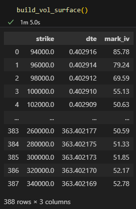
def build_vol_surface(currency="BTC"):
    """
    Builds a volatility surface dataset for call options of the specified currency.

    Parameters:
    currency (str): The asset symbol (e.g., "BTC", "ETH").

    Returns:
    pd.DataFrame: A DataFrame with columns ['strike', 'dte', 'mark_iv'].
    """
    instruments = get_instruments(currency)
    rows = []

    for inst in instruments:
        if inst["option_type"] != "call":
            continue

        ticker = get_ticker(inst["instrument_name"])

        mark_iv = ticker.get("mark_iv", None)
        if mark_iv is None:
            continue
        
        expiration = pd.to_datetime(inst["expiration_timestamp"], unit='ms', utc=True)
        now = pd.Timestamp.now(tz='UTC')
        delta = expiration - now
        dte = round(delta.total_seconds() / (24 * 60 * 60), 3)

        rows.append({
            "strike": inst["strike"],
            "dte": dte,
            "mark_iv": mark_iv
        })

    return pd.DataFrame(rows)

def build_front_expiry_smile(currency="BTC"):
    """
    Builds a DataFrame containing only front expiry (DTE<1) call options IV data.

    Parameters:
    currency (str): The currency symbol (e.g., "BTC", "ETH").

    Returns:
    pd.DataFrame: Filtered DataFrame with columns ['strike', 'dte', 'mark_iv'] for front expiry.
    """
    vol_surface = build_vol_surface(currency)

    front_expiry_df = vol_surface[vol_surface["dte"] == min(vol_surface["dte"])].sort_values("strike")

    return front_expiry_df

This gives us the following dataframe if we run build_vol_surface():

Here are the functions for plotting the whole volatility surface and just the front expiry volatility smile:

def plot_vol_surface(df):
    """
    Plots a 3D volatility surface using strike price, days to expiry (DTE), and implied volatility.

    Parameters:
    df (pd.DataFrame): DataFrame containing columns 'strike', 'dte', and 'mark_iv'.
    """
    fig = plt.figure(figsize=(10, 7))
    ax = fig.add_subplot(111, projection='3d')

    # Pivot data into grid
    X = df['strike']
    Y = df['dte']
    Z = df['mark_iv']

    # Convert to numpy arrays
    xi = np.linspace(X.min(), X.max(), 40)
    yi = np.linspace(Y.min(), Y.max(), 40)
    xi, yi = np.meshgrid(xi, yi)

    zi = griddata((X, Y), Z, (xi, yi), method='linear')

    surf = ax.plot_surface(xi, yi, zi, cmap='viridis', edgecolor='none')
    ax.set_xlabel('Strike Price')
    ax.set_ylabel('Days to Expiry')
    ax.set_zlabel('Implied Volatility (%)')
    ax.set_title('Deribit Volatility Surface')
    fig.colorbar(surf, shrink=0.5, aspect=5)
    plt.tight_layout()
    plt.show()

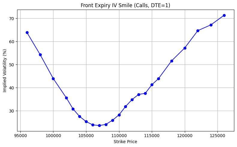
def plot_front_expiry_smile(df):
    """
    Plots the IV smile.

    Parameters:
    df (pd.DataFrame): DataFrame returned by build_front_expiry_smile().
    """
    plt.figure(figsize=(8, 5))
    plt.plot(df["strike"], df["mark_iv"], marker='o', linestyle='-', color='blue')
    plt.title("Front Expiry IV Smile (Calls, DTE<1)")
    plt.xlabel("Strike Price")
    plt.ylabel("Implied Volatility (%)")
    plt.grid(True)
    plt.tight_layout()
    plt.show()

Let’s run both:

df = build_front_expiry_smile("BTC")
plot_front_expiry_smile(df)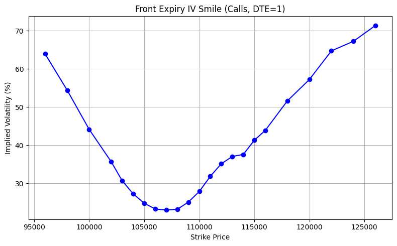

df = build_vol_surface("BTC")
plot_vol_surface(df)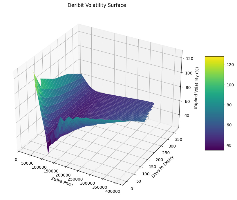

There is something interesting going on with the volatilite surface: The further out you go in expiry the flatter it becomes (We do know that longer term returns tend to become more normal) and the more significant the skew seems to become.

---

How to Model the Volatility Smile

Let’s say you wanted to predict changes in the volatility smile (which we will do later in this article). Do we keep track of every single option? No, that would be way too many parameters to keep track of and would potentially make things much more noisy. This reason and because the shape of the volatility smile isn’t all that complicated leads us to using a parameterization to describe the smile.