Kelly Criterion in Practice

How it works and how a real desk would use it

Dec 19, 2025

If you’ve been lurking in quant forums for a while, I bet you’ve come across a conversation like this before:

A: “Kelly is too dangerous, use half-kelly instead!”
B: “No use 0.75x Kelly, 0.5x is too low!”
C: “Actually, you should use this formula for continuous Kelly!”

In this article, we will delve into the actual math of Kelly, rather than relying on word-of-mouth.

Thanks to the amazing support of our premium readers, we are able to release an article for free from time to time.
If you wish to unlock over 50 premium articles like this one, as well as 3 articles per month, consider supporting us as well!

The Kelly Objective — What Are We Even Optimising?
Classic Kelly — Model and Closed-Form Solution
Fractional Kelly — What’s the point?
A Bounded-Below Model — The Impact of Tail Risk
A Quadratic Approximation — The Dangerous Formula You Find Online
Continuous-Time Kelly (GBM) — Moving On From Discrete Models
Multi-Asset Continuous-Time Kelly — When We Trade Multiple Assets
Estimation Error: Bayesian Approach — Updating Your Beliefs of Odds
Dynamic Sizing — Don’t Use Constant Kelly!
Final Remarks — Final Remarks and Discord

The Kelly Objective — What Are We Even Optimising?

We start with some notation.
Let:

r = per-period risk-free simple return
X_{t+1} = per-period excess simple return of the risky asset
f = dollar exposure to the risky asset, as a fraction of current wealth (f=1 means fully invested; f>1 means levered; f<0 means short)

Then discrete-time wealth evolves as:

$W_{t+1} = W_t(1 + r + fX_{t+1})$

The Kelly objective that we want to maximize is the per-period expected log growth:

$g(f) = \mathbb{E}[\log(1+r+fX)]$

Working with the log of wealth has a couple of nice properties:

log(0) = -inf, going bankrupt is unacceptable.
Maximizing E[log(1+R)] maximizes the long-run growth rate of wealth.
Log utility represents risk aversion: Going from $1000 → $2000 is much nicer than going from $10.000 → $11.000.

g(f) is an expected value, and we know that log(0) is -inf, so for g(f) to be finite we have the necessary condition:

$\mathbb{P}(1+r+fX \leq 0) = 0$

This also explains why you can’t use an unbound normal distribution to model your returns, since even if the probability of getting a return that wipes out your portfolio is astronomically small, the expected value (g(f)) will be -inf.

Classic Kelly — Model and Closed-Form Solution

Let’s start with a super simple binary model:

Win probability: p
Lose probability: q = 1-p
Odds: risk 1, win b

By betting a fraction f of wealth, our new wealth will be multiplied by:

Win: 1 + bf
Lose: 1 - f

The Kelly objective g(f) will now look as follows:

$\begin{align} g(f) &= \mathbb{E}[\log(1+fX)] \\ &= p \log(1+fb) + q\log(1-f) \end{align}$

We can find a closed-form solution for f that maximizes g by taking the derivative and setting it to 0:

$\begin{multline} \frac{dg}{df} = \frac{bp}{bf+1} - \frac{q}{1-f} \\ \frac{dg}{df} = 0 \iff f = \frac{pb-q}{b} \end{multline}$

This gives us the traditional formula for the Kelly fraction:

$f^* = \frac{pb-q}{b}$

Let’s code this up!

First, some imports and configs that we will use in this project:

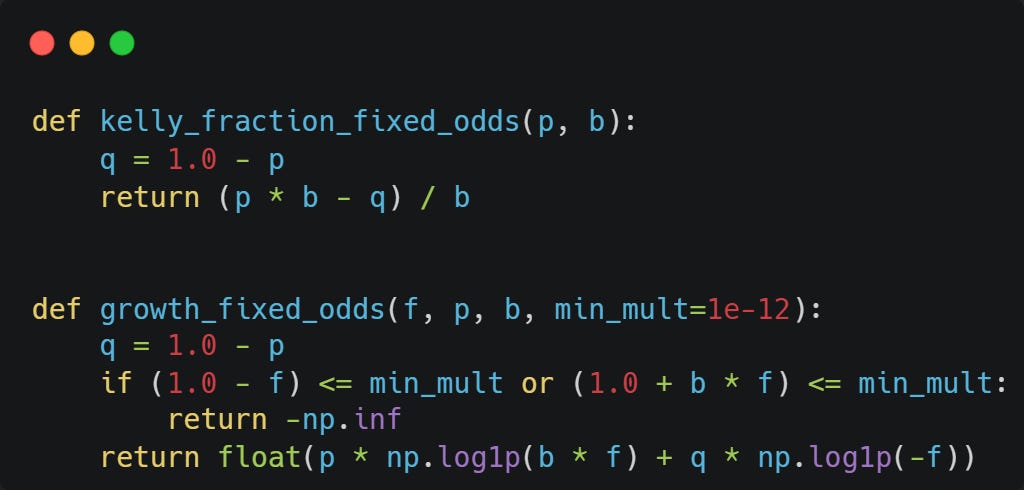
Now the code to compute the Kelly fraction and the expected log growth:

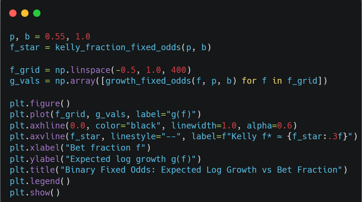
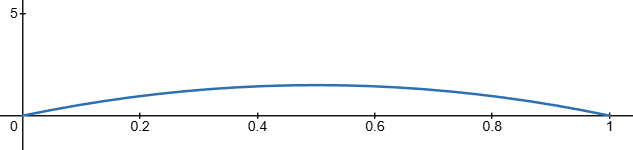
With p = 0.55 and b = 1.0, we obtain a Kelly fraction of 0.1, meaning we should bet 10% of our entire wealth on this every time.

We can verify that this is correct using a plot:

Fractional Kelly — What’s the point?

There is one biiiig problem with the Kelly fraction: it just barely avoids ruin.
At the Kelly fraction f, our probability of ruin is 0 almost surely. Any increase in f above Kelly gives a positive probability of eventual ruin.

If you overestimated your probability of winning, then even Kelly will give you a leverage that gives you a non-zero probability of eventually going to 0.

So the intuitive idea of just using a fraction of Kelly is actually pretty sound, although the execution isn’t the best (we will get to this later).

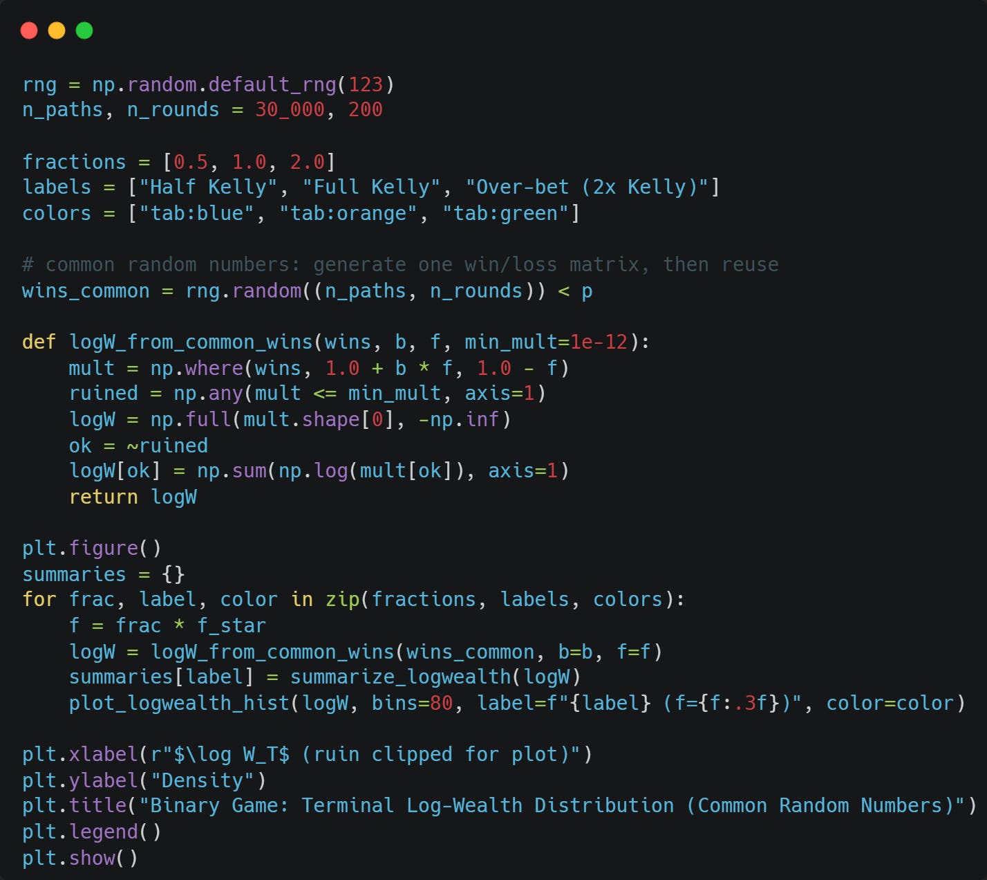
Let’s compare what happens at Half Kelly, Full Kelly, and Double Kelly.
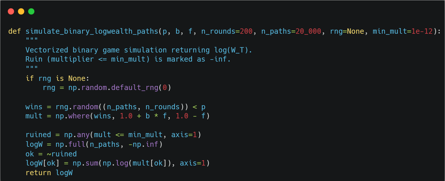
The following function will simulate the binary game with probability of winning p, a payout b, and leverage f:

To better compare the 3, I will use the same random numbers in all 3 simulations:

A Bounded-Below Model — The Impact of Tail Risk

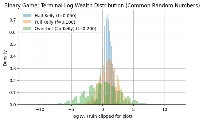
We usually only have samples of excess return x_i available.
We can then approximate the Kelly objective g via:

$g(f) \approx \frac{1}{n} \sum_{i=1}^n \log(1 + r + fx_i)$

where n is the number of samples available.

We maximize over a feasible interval where 1+r+fx_i > 0 for all samples.
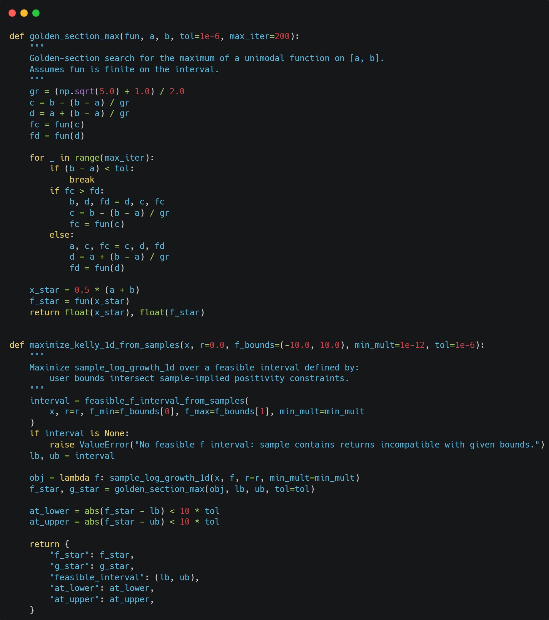
To compute g from samples and to compute the feasible interval, we can use the following functions:

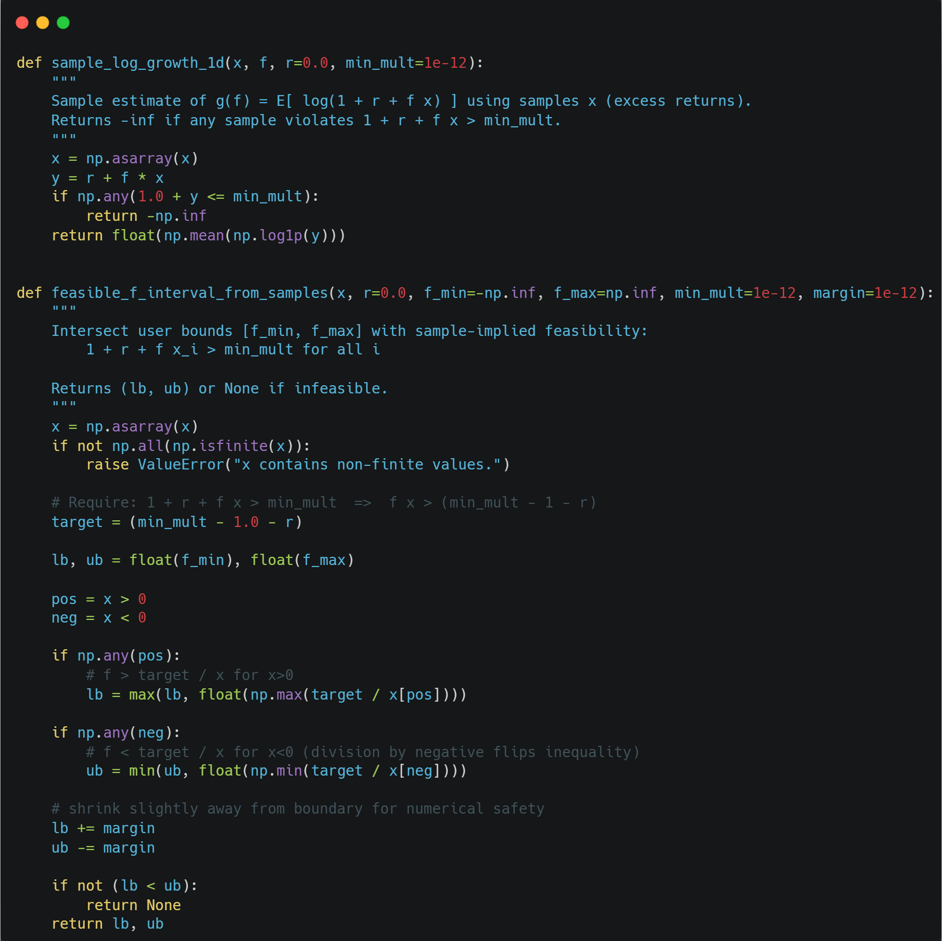
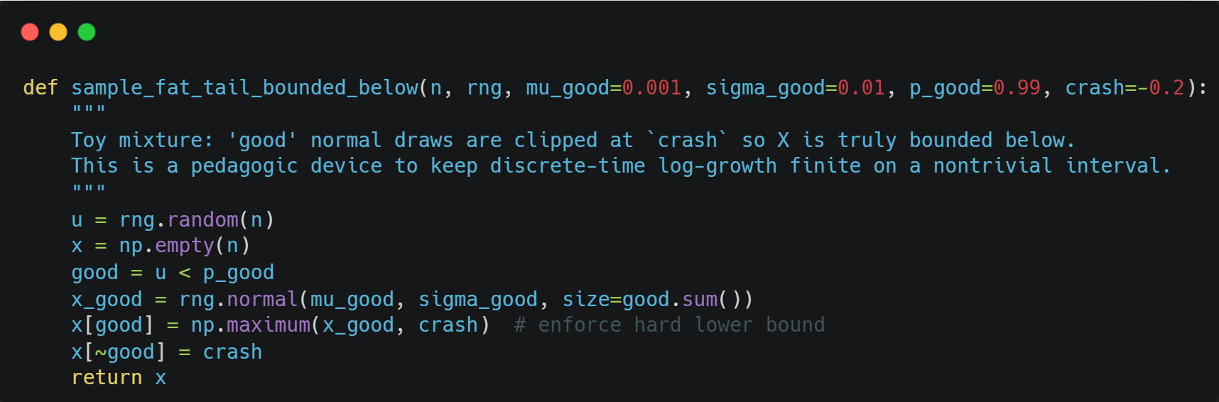
To illustrate how much of an impact tail risk has on Kelly, consider the following scenario:

With probability p_good: Sample normal returns, clipped at a crash floor.
With probability 1-p_good: Sample a fixed crash x_crash (a point mass at the floor)

We can sample those returns with the following function:

We can maximise the log growth rate (Kelly objective) on our feasible interval using golden section search:

I talked about the golden section search in more detail in the following article:

Statistical Arbitrage on Uniswap v3 (Full Strategy)

Vertox and BowTiedDevil

Aug 20

Statistical Arbitrage on Uniswap v3 (Full Strategy)

The Statistical Arbitrage Series is a collaboration between Vertox and BowTiedDevil to present stat arb strategies and their application in a blockchain environment.

Read full story

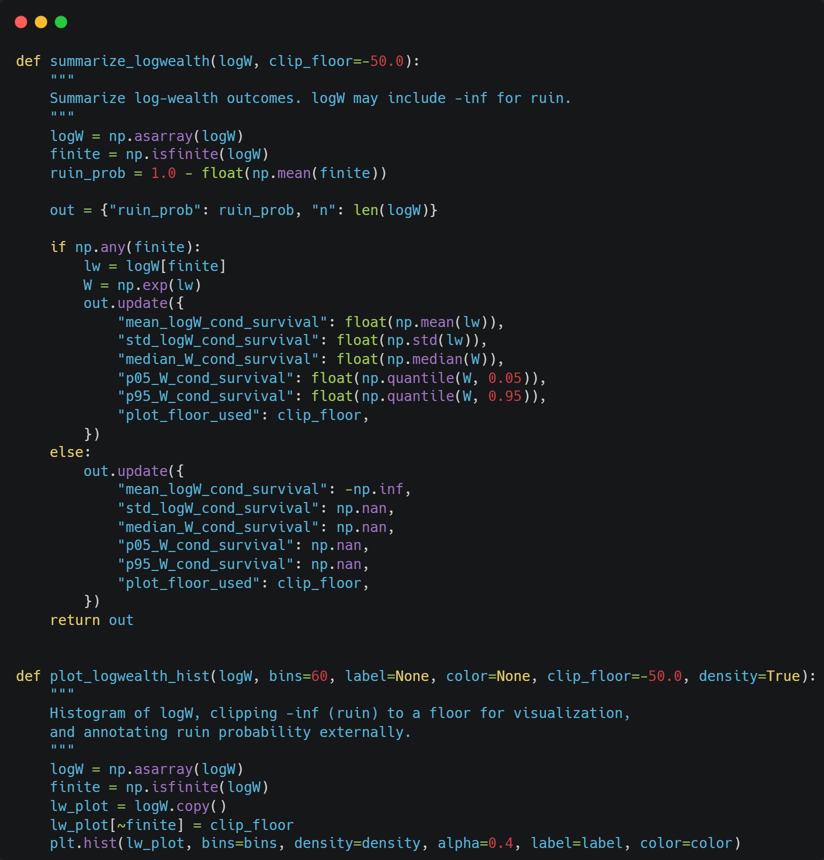
We will further use the following two functions to summarize information about log wealth:

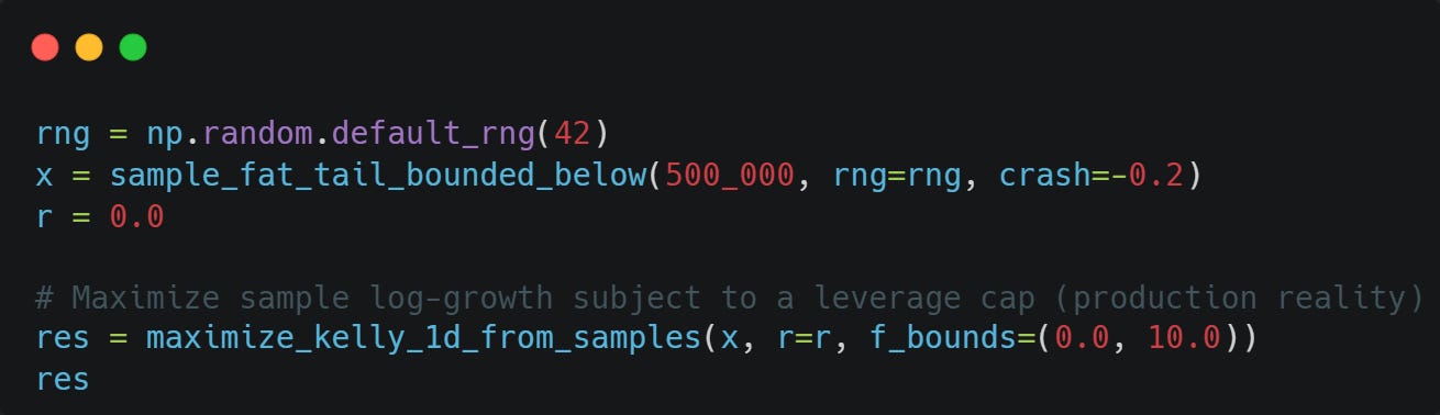
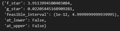
Let’s sample from our bounded fat-tailed distribution now and find the optimal fraction to bet:

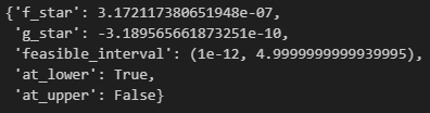
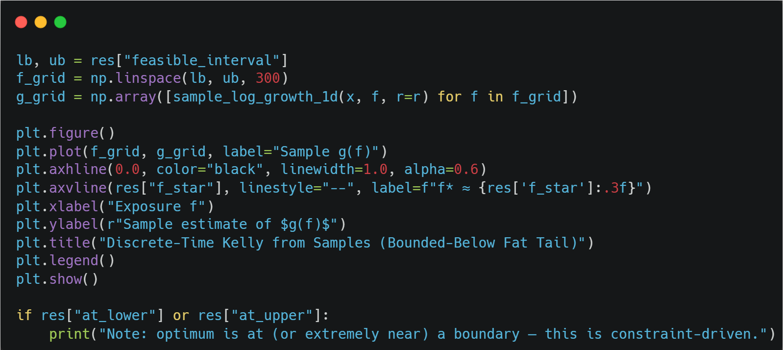
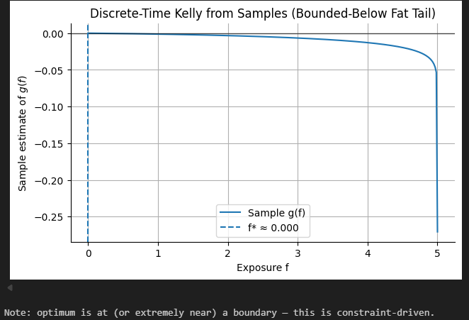
As you can see, we shouldn’t be betting at all.
Let’s see what happens if we increase the mean of the normal distribution from 0.1% to 1%:

Much better, but we are also pretty close to the leverage that will cause us to reach ruin with probability 1 almost surely.

A Quadratic Approximation — The Dangerous Formula You Find Online

Recall the formula for the Kelly objective:

$g(f) = \mathbb{E}[\log(1+r+fX)]$

The Taylor expansion of log(1+y) around y = 0 is:

$\log(1+y) = \sum_{n=1}^\infty (-1)^{n+1} \frac{y^n}{n} = y - \frac{y^2}{2} + \frac{y^3}{3} + \frac{y^4}{4} + ...$

The Second-order approximation is therefore:

$\log(1+y) \approx y - \frac{y^2}{2}$

Substitute y = r+fX, then:

$\log(1+r+fX) \approx (r + fX) - \frac{(r+fX)^2}{2} = r - \frac{r^2}{2}+ fX(1-r) - \frac{f^2X^2}{2}$

Taking expectation on both sides, we finally obtain (since r and f are constants):

$\mathbb{E}[\log(1 + r + fX)] \approx r - \frac{r^2}{2} + f\mathbb{E}[X](1-r) - \frac{f^2}{2}\mathbb{E}[X^2]$

Now we simplify r - r^2/2 using the second-order approximation of log(1+r) and factor out the (1+r) term to finally obtain:

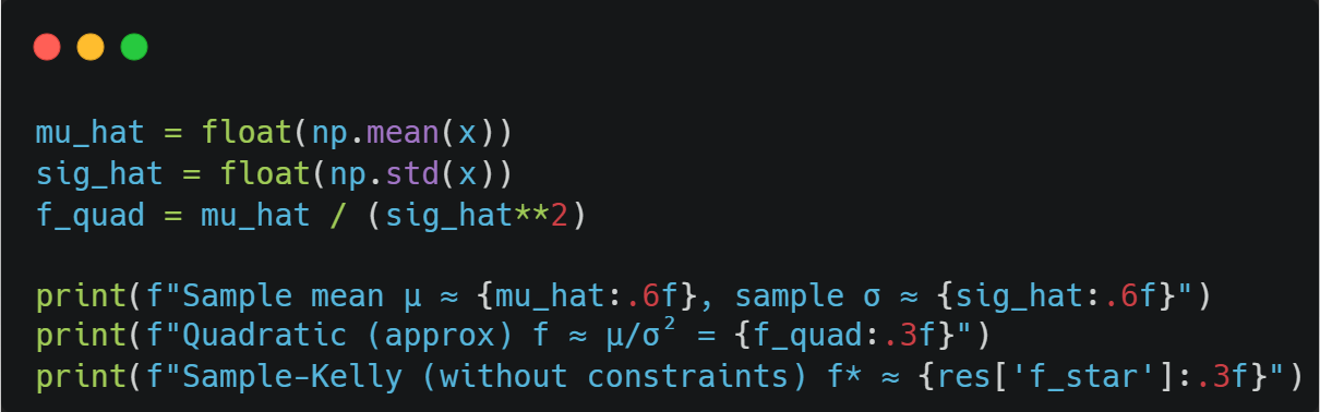
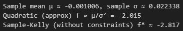
$\mathbb{E}[\log(1+r+fX)] \approx \log(1+r) + \frac{f\mathbb{E}[X]}{1+r} - \frac{1}{2} \frac{f^2\mathbb{E}[X^2]}{(1+r)^2}$

A very naive formula I’ve seen online now further assumes r ≈ 0 and E[X^2] ≈ sigma^2.
With this, we get the final formula:

$\mathbb{E}[\log(1+r+fX)] \approx f\mu - \frac{f^2 \sigma^2}{2}$

Where mu = E[X].

To find the f that maximises this, we take the derivative and set it to 0:

$\frac{d}{df}[f\mu - \frac{f^2\sigma^2}{2}] = \mu - f\sigma^2 = 0$

This has the following solution that you often see online:

$f^* \approx \frac{\mu}{\sigma^2}$

We’ve done so many approximations and assumptions here. This formula becomes extremely unreliable in real markets.

Here is what this approximation would have given us on our fat-tailed samples:

Continuous-Time Kelly (GBM) — Moving On From Discrete Models

One really nice property of continuous-time models is that we avoid the discrete-time “one-step wipeout” issue because the wealth process stays strictly positive under diffusion dynamics.

Let’s model a risky asset with excess drift mu via Geometric Brownian Motion:

$\frac{dS}{S} = (r+\mu)dt + \sigma dB_t$

Let’s say we have wealth W and maintain constant exposure f to the risky asset.
Our wealth changes from two sources:

Cash portion (1-f)*W earns r.
Risky asset portion f*W follows the asset’s dynamics.

Our wealth return dynamics are therefore:

$\frac{dW}{W} = r dt + f\mu dt + f\sigma dB_t$

What we care about are the dynamics of log wealth, however.
We can apply Itô’s lemma to obtain:

$d(\log(W)) = [r + f\mu - \frac{1}{2}f^2 \sigma^2]dt + f\sigma dB_t$

The drift component of log wealth is:

$\gamma(f) = r + f\mu - \frac{1}{2}f^2\sigma^2$

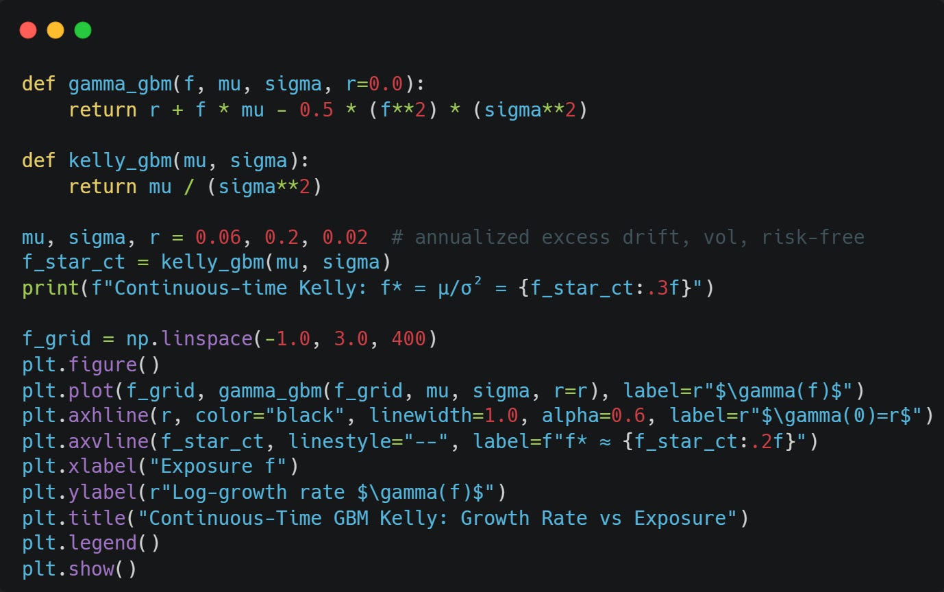
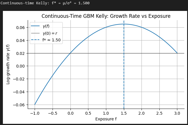
To maximize the drift of log wealth, we again take the derivative of this with respect to f and set it equal to zero (you know the drill) to obtain:

$f^* = \frac{\mu}{\sigma^2}$

That’s the same formula we obtained in our second-order approximation!

Let’s code it up and confirm our formula is correct:

Multi-Asset Continuous-Time Kelly — When We Trade Multiple Assets

Why limit ourselves to one asset when we can trade multiple assets at once?

Let X be the vector of excess returns in continuous time with drift mu and covariance Sigma. We have the multivariate Gaussian Process:

$dX = \mu dt + \Sigma^{1/2} dB_t$

Doing the same process as in the previous section, we arrive at the drift of our log wealth:

$\gamma(w) = r + w^T \mu - \frac{1}{2}w^2\Sigma w$

with weights w.

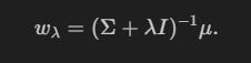
The Kelly solution is:

$w^* = \Sigma^{-1} \mu$

Let’s compute and verify this:

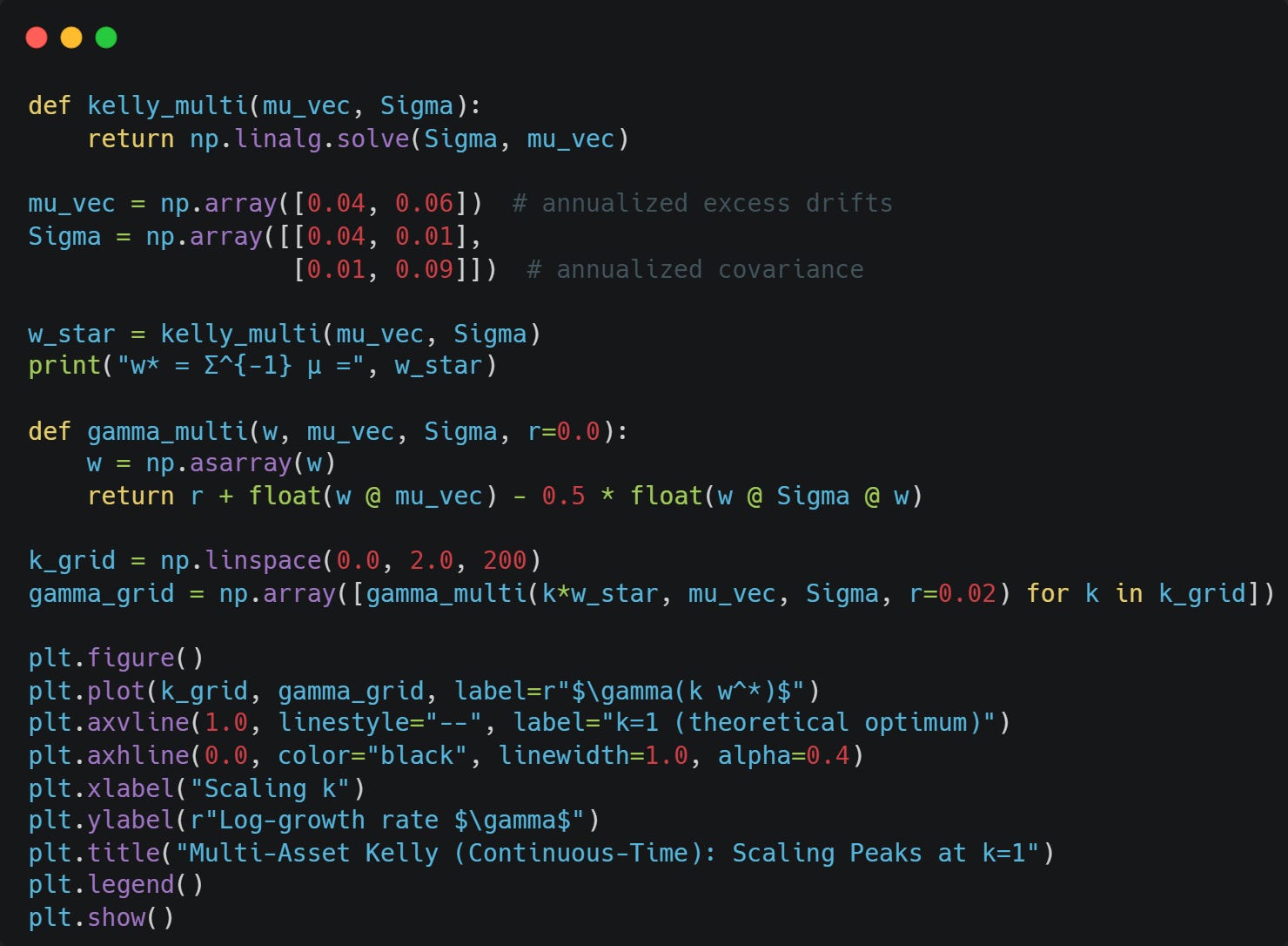
There is one major issue with the Kelly solution (besides the fact that markets don’t follow Brownian motion): Sigma^-1 is extremely unstable. Covariance matrices are nearly singular for correlated assets, making small changes to Sigma can give you a vastly different Sigma^-1.

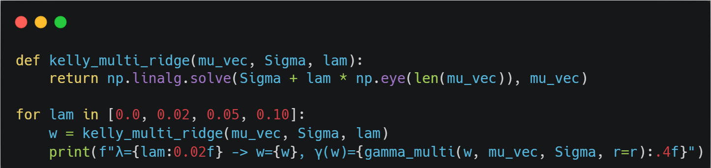
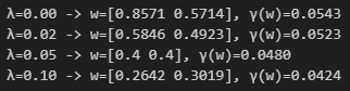
Our goal is to reduce the variance by introducing some bias. A simple way to do this is using Ridge Regularisation:

I talk in more detail about regularisation in the following article:

Avoiding Overfitting and Colinearity with Regularization

Vertox

May 5

Avoiding Overfitting and Colinearity with Regularization

2 of the most common problems we face when building trading models are overfitting and colinearity. Regularization is a technique that we can use to combat both of those problems.

Read full story

What you need to know here is: The more we increase lambda, the more our weights will shrink towards zero (more bias), but the smaller the variance will be.

Here is the impact of different values of lambda on our weights:

Estimation Error: Bayesian Approach — Updating Your Beliefs of Odds

Imagine you are walking around in Las Vegas, and someone in an alley calls you to play a game. Because you have no survival instincts, you decide to give it a try. He suggests throwing a coin. If you win, your payout is b=1. If he wins, his payout is 1.

You believe the nice gentleman is using a fair coin, but you are sceptical. Your prior belief on the win probability is a Beta(a0, b0) distribution with a0 = 2 and b0 = 2. This is a symmetric distribution centred at p=0.5:

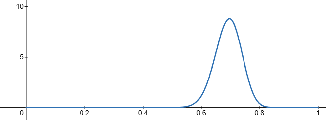
You guys decide to play 100 games, and he wins 70 times… You no longer believe the coin is fair and update your beliefs about the probability of him winning. Your new posterior distribution looks as follows:

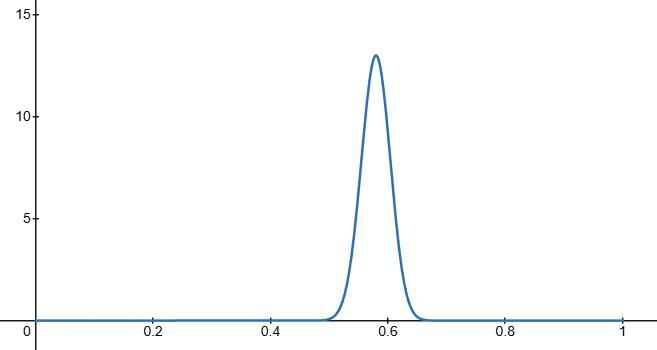
You still decide to play another 300 games, and this time he only wins 162 times.
Your new posterior distribution now looks as follows:

The process we just did is called Bayesian inference, where we compute the posterior probability according to Bayes’ theorem:

$\mathbb{P}(H|E) = \frac{\mathbb{P}(E|H)\mathbb{P}(H)}{\mathbb{P}(E)}$

where:

H is a hypothesis whose probability you are trying to estimate.
P(H) is your prior probability for the hypothesis.
E is the evidence you collect by playing.
P(H|E) is the posterior probability. The probability of H with new evidence E.

Our prior is a Beta(a0, b0) distribution. The density is:

$\pi(p) \propto p^{a_0-1}(1-p)^{b_0-1}=p(1-p)$

We observe n=100 trials with k=70 wins. The likelihood is binomial:

$\mathcal{L}(p|\text{data}) = {70\choose100}p^{70}(1-p)^{30}$

According to Bayes’ Theorem, we have:

$\pi(p|\text{data}) \propto \pi(p) \times \mathcal{L}(p|\text{data})$

Substituting:

$\pi(p|\text{data}) \propto p(1-p) \times p^{70}(1-p)^{30} = p^{71}(1-p)^{31}$

This is the kernel of a Beta distribution:

$p|\text{data} \sim \text{Beta}(a_0 + k, b_0 + n - k)$

So after our first round of 100 games, our posterior distribution is Beta(72,32).

Note: The mean of a Beta(a,b) distribution is a/(a+b).

We are gonna test 4 betting strategies against the mysterious alley guy now. For all 4 strategies we start by playing 100 test games to get an idea of the true probability of heads and tails.

We estimate p as the fraction of games won. We then bet using Kelly: f = 2p-1.
Same as strategy 1, but we bet with half-Kelly.
We use our Bayesian inference strategy and bet with Kelly using the mean of our posterior distribution as the probability.
We use Bayesian inference like in strategy 3, but use the 10th percentile of our posterior distribution instead of the mean.

Here is all of that coded up:

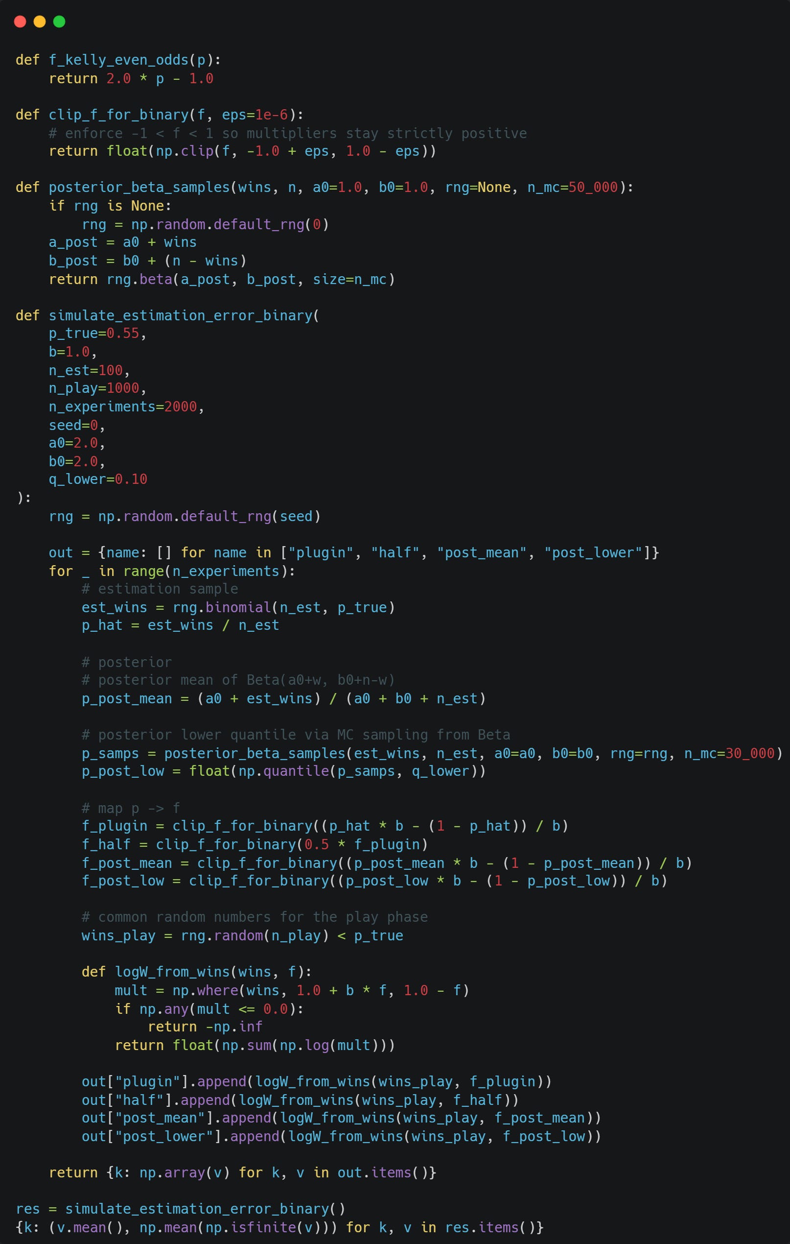
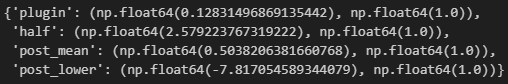
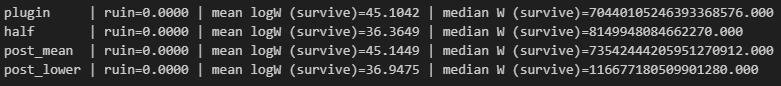
Half Kelly has the highest mean log wealth growth, and no strategy ever went bankrupt.

If we increase our warmup games to 1000 and then play 10000 games in total (across 20000 experiments), those numbers change:

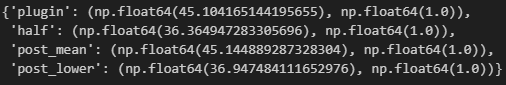
The more optimal strategies start to outperform!

Here are the distributions of the final log wealths:

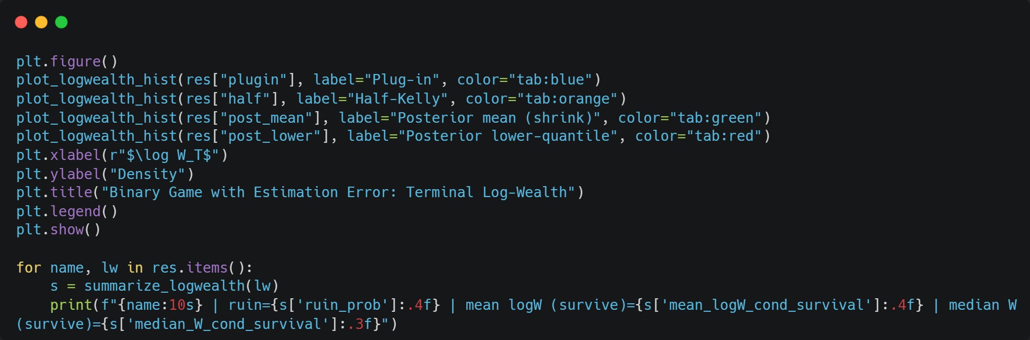
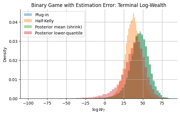
Note: The true probability of us winning was 55% (Thank you, mysterious coin guy!).

Dynamic Sizing — Don’t Use Constant Kelly!

An even better strategy would be to update your posterior distribution in the Bayesian inference strategy after every single game (or every few games).
There is a small problem with this, though: what if the true probability of winning changed over time? The more games we played, the slower Bayesian inference updates.

There are a few major ways to solve this issue:

Use a sliding window and only use the last N observations for your inference.
Weight recent data more heavily.
Monitor for regime changes and reset when detected.

Those are left as an exercise to the reader.

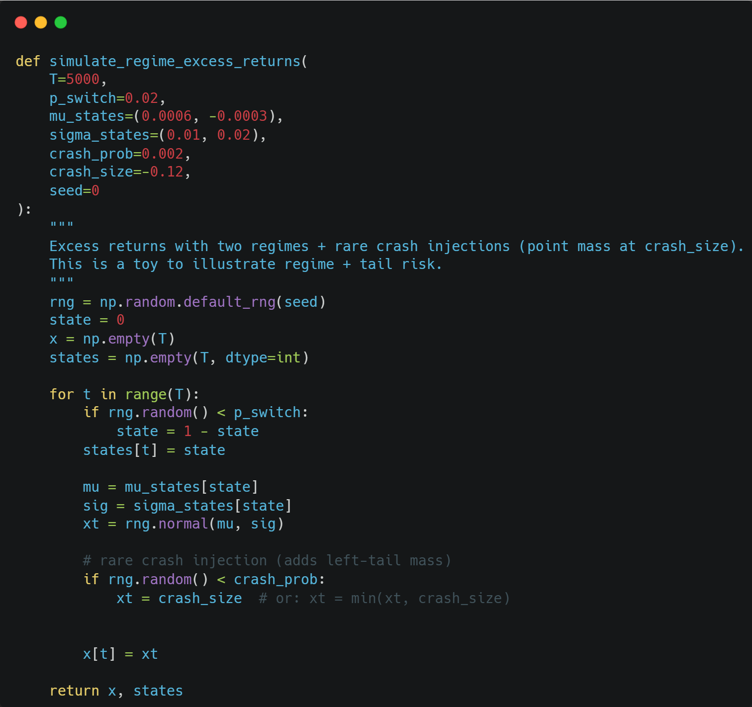
Imagine the shady alley man actually has 2 coins now that he switches between at random, and instead of flipping a coin, he samples from a normal distribution. Further, with a small probability, we get a crash.

We can simulate this with the following code:

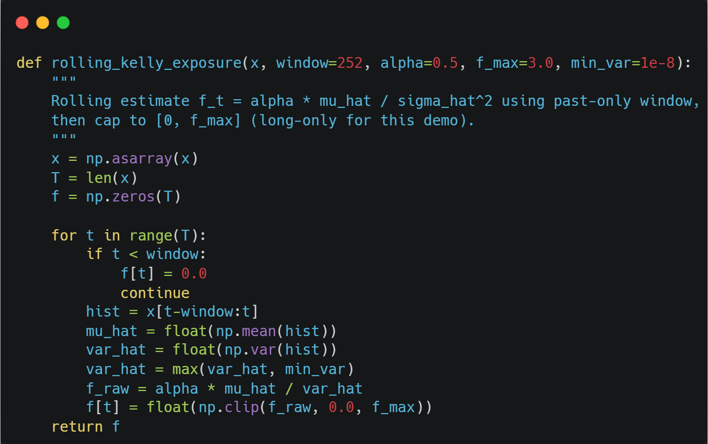
We are gonna use a rolling window to bet with Kelly and hopefully adapt to the changing regimes:

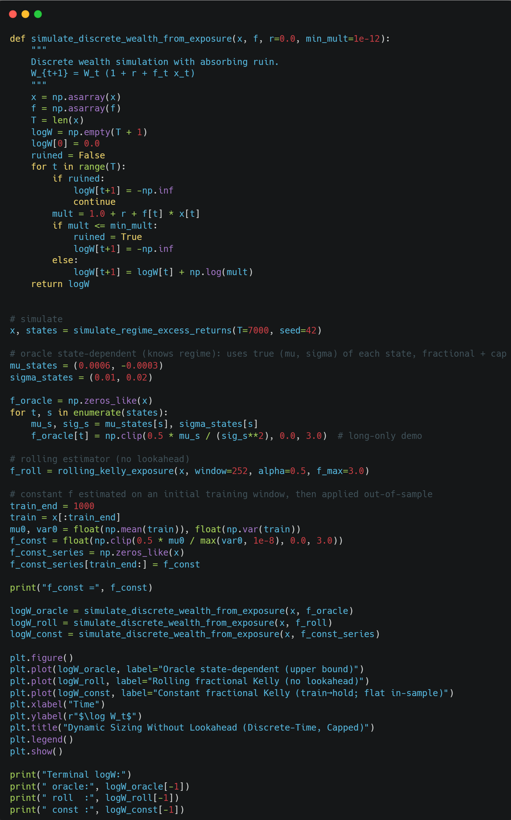
Let’s test out 3 different strategies now:

A crystal ball that knows what regime we are in and knows all the true probabilities to bet optimally using Kelly.
Our rolling Kelly.
Play a couple of warm-up games and then play with fixed Kelly.