Market Making Models

An overview of the literature

We’ve all heard those 2 names being dropped before: Avellaneda & Stoikov.
Whenever those names drop it’s about the market making model from their paper High-frequency trading in a limit order book.

Beyond that you don’t really hear about other market making models all that often even though the A&S model is really limiting.

In this article I’m gonna be summarizing results of some popular market making papers.

---

Table of Content

1. Utility Functions

2. Avellaneda & Stoikov

3. Fitting the Model Parameters

4. Inventory Based Models

5. Information Based Models

6. Guéant–Lehalle–Fernandez-Tapia

7. Market Making with Alphas

8. Cartea-Jaimungal

9. Cartea-Jaimungal-Ricci

10. Final Remarks

---

Utility Functions

Before we can understand how all those market making models are derived we need to understand utility functions.

What they do is measure satisfaction. Here is an example:

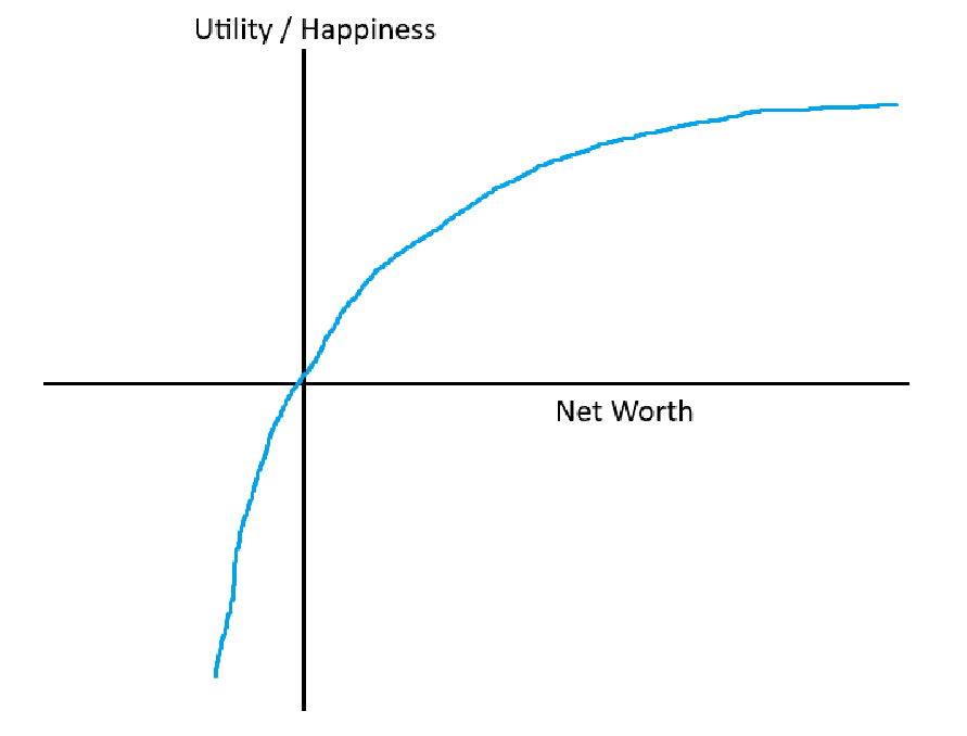
We don’t have a linear relationship between net worth and happiness, eventually it flattens out.
Here is one utility function that avellaneda & stoikov use for example:

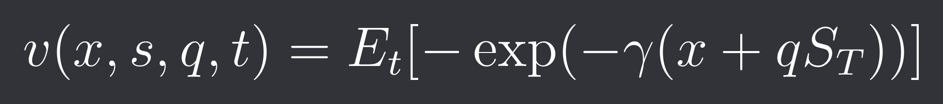
specifically, it’s the expected exponential utility.

The different variables here are:

• x: initial wealth

• s: initial asset price

• q: inventory

• t: time

• gamma: risk aversion parameter

• S_T: asset price at expiry

This can be written as:

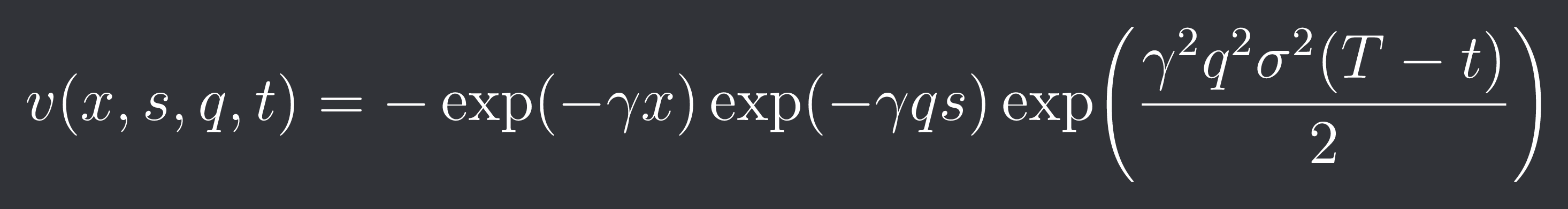
This is the utility of a market participent without any limit orders that just holds q assets until expiry T.

Note: If you are market making on something like perps then this (T-t) factor disappears as you don’t have an expiry.

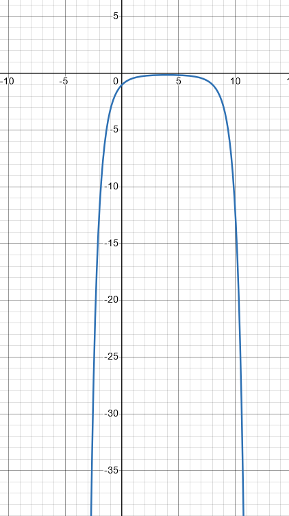
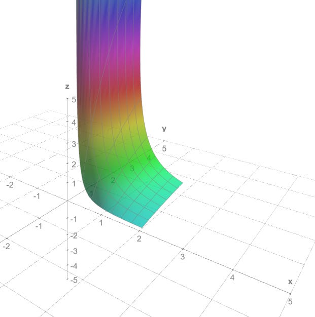
Here is what this utility function could look like for locked values of x, s, t, gamma and sigma but different values of q:

---

Avellaneda & Stoikov

Using this expected exponential utility they now define the so called “reservation” bid and ask price.

The reservation bid price is the price at which the agent wouldn’t mind having one more asset in his inventory (Same utility).
The reservation ask price is the price where he wouldn’t mind one less asset.

So:

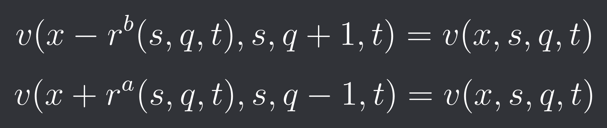
We can plug both into the equation for v and then solve for r^b and r^a:

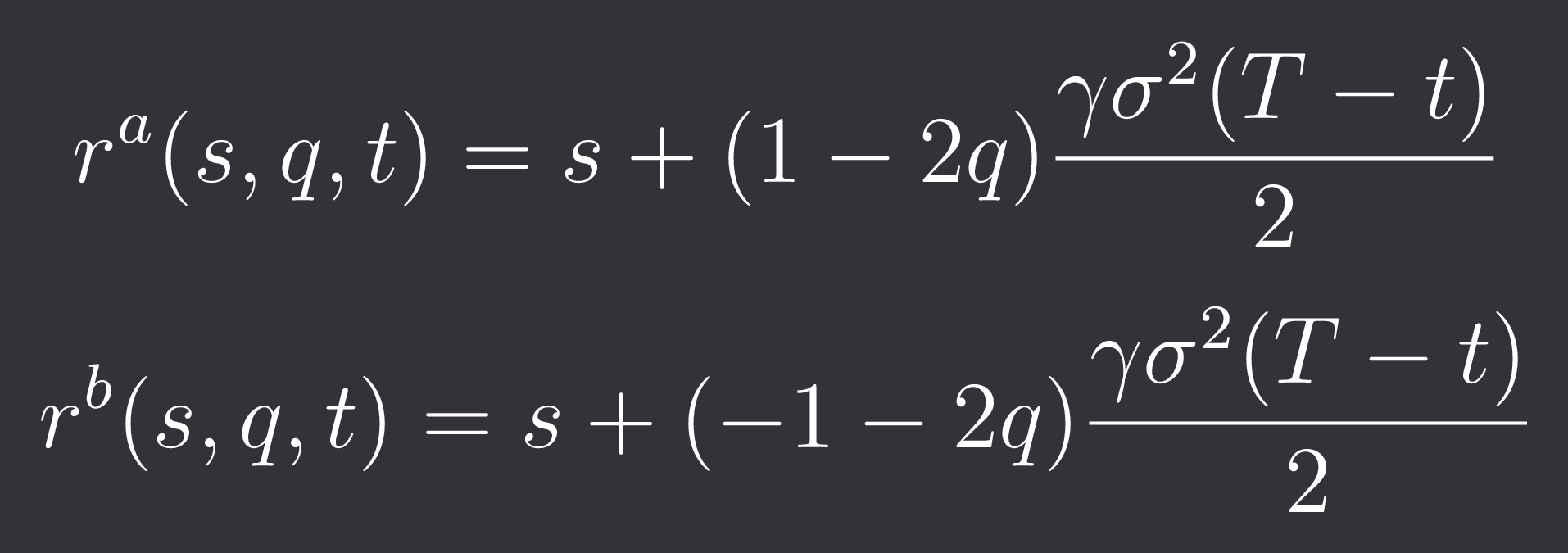
The midprice of this ((r^b + r^a)/2) will be called the reservation price.

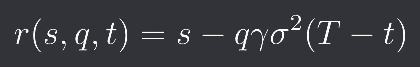
As you can see it’s an adjusted midprice of the asset given our inventory.
The more inventory we put on the more we skew our midprice to get rid of the inventory.
Also the more risk averse we are, the more volatile the market is and the more time until expiry is left the more we skew our midprice.

A lot of math later which I will not discuss in this post we get the following equation for the bid-ask-spread:

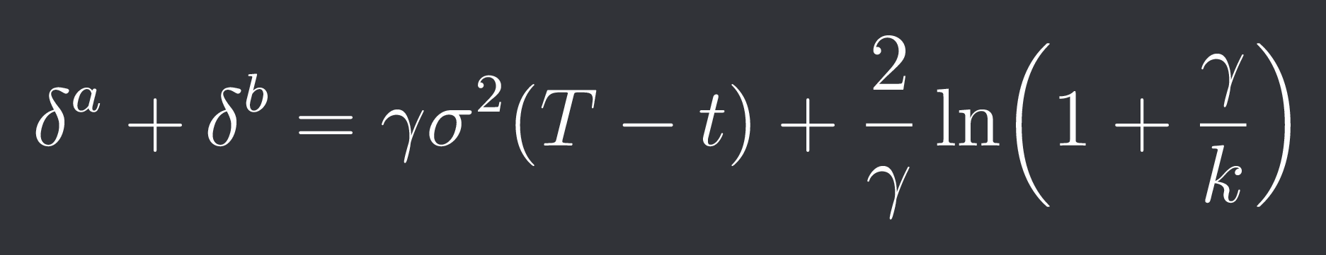
Here k is a parameter that represents the liquidity of the asset.
As you can see the right hand side of the equation is a constant, the minimum spread at which we quote and it depends on the liquidity of the asset and our risk aversion.

Here is the minimum quoting distance for different gammas (x) and deltas (y).

The left term also makes sense. The more risk averse we are the wider we quote and the more volatile the market is and the more time left the wider we quote as well.

---

Fitting the Model Parameters

So we have the parameters gamma and k for risk aversion and liquidity but… what should we choose them to be? 0.1? 4? 100?

Let’s start with the liquidity parameter k first.

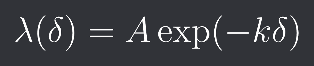
The paper assumes that the rate at which orders are executed at distance (spread) delta away from the midprice follows:

One paper that described the process of fitting this k and A parameter is the following: http://events.chairefdd.org/wp-content/uploads/2013/06/CAHIER_MICRO_1.pdf.

We are more interested in figuring out what value to use for our risk aversion parameter though as that is an arbitrary parameter.

For this we will run some historical simulations for our inventory given different values of gamma and see what the profitability and volatility of our portfolio is like.

I will use 1 day of data but in practice you wanna use much more than that.

We are also gonna assume that our size is so small that we have no market impact, otherwise simulation becomes a reaaaaal challange.

quotes = pd.read_csv("binance-futures_quotes_2024-08-01_BTCUSDT.csv").set_index("timestamp")[['ask_price', 'bid_price']]
quotes.index = pd.to_datetime(quotes.index*1000)
quotes = quotes.groupby(quotes.index).last()
quotes['mid_price'] = (quotes['bid_price'] + quotes['ask_price'])/2

trades = pd.read_csv("binance-futures_trades_2024-08-01_BTCUSDT.csv").set_index("timestamp")[['side', 'price']]
trades.index = pd.to_datetime(trades.index*1000)
trades = trades.groupby(trades.index).last()

df = pd.concat([quotes[['mid_price']], trades], axis=1).sort_index()
df[['mid_price']] = df[['mid_price']].ffill()
df.dropna(inplace=True)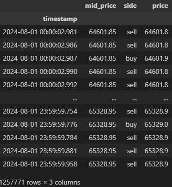

I’m gonna use the following constants:

• k=1.5

• sigma^2 = 800

Here is what we get for gamma=0.01:

k = 1.5
sigma = 800
gamma = 0.01

inventory = [0]
reservation_price = [df['mid_price'].iloc[0]]
spread = gamma * sigma + (2/gamma)*np.log(1 + gamma/k)

for i in range(len(df)):
    if df['price'].iloc[i] <= reservation_price[-1] - spread/2:
        inventory.append(inventory[-1] + 1)
    elif df['price'].iloc[i] >= reservation_price[-1] + spread/2:
        inventory.append(inventory[-1] - 1)
    else:
        inventory.append(inventory[-1])

    reservation_price.append(df['mid_price'].iloc[i] - inventory[-1]*gamma*sigma)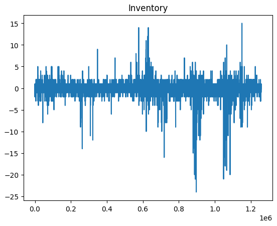

and inventory returns:

inventory_rets = df['mid_price'].pct_change(1) * inventory[:-1]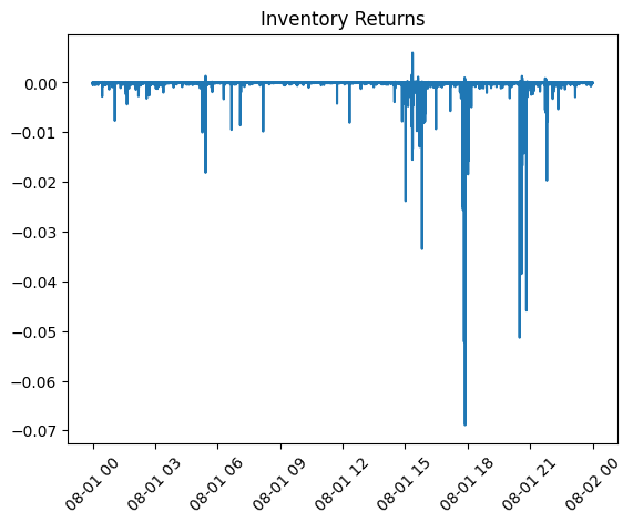

Now let’s get the standard deviation and sum of that for different values of gamma and plot it:

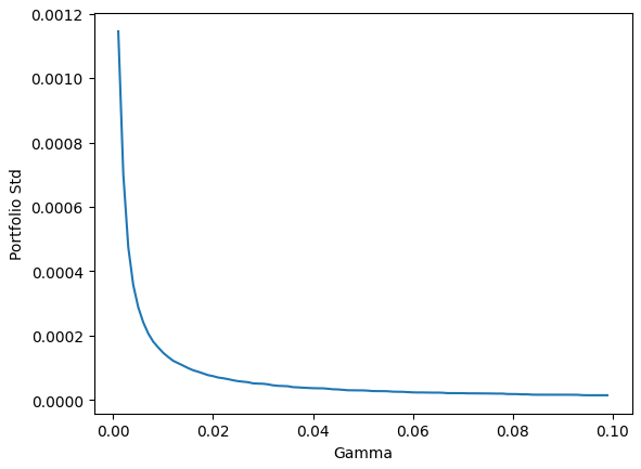
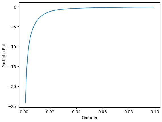
Like expected a simple Avellaneda & Stoikov Market Making model is unprofitable no matter the risk aversion parameter.

We might as well plot pnl/std (almost sharpe) tho:

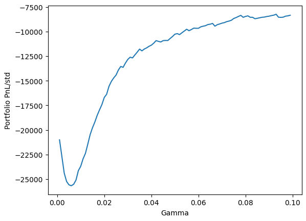
Note: This is before fees so this will look even worse in reality.

So for everyone that is planning on running an A&S Market Maker: Maybe reconsider that! (At least for BTC in Binance. I know I know I couldn’t have chosen something more competitive than that)

If we were profitable we would choose a gamma where we are happy with the profit given the level of volatility or we’d maximize a metric like the sharpe ratio.

---

Inventory Based Models

Inventory-based models focus on the risk associated with the inventory a market maker puts on.

Ho and Stoll Model

The Ho and Stoll Model is an inventory-based market making model.

They make the following assumptions: