
Option Pricing Basics
Risk neutral valuation and discrete models

An options contract gives the buyer the right to buy or sell (call or put) the underlying asset at an agreed upon price and time.
With european options we only have that right at expiration while with american options we have the right before expiry as well making american options harder to price. Whenever we don’t explicitly talk about american options in this article you can assume that we are talking about european options.
Well if I want to buy the right to buy BTC at $100.000 on 01/03/2025, how much should that be worth? This is what option pricing models tell you!
There are a lot of misconceptions when it comes to options pricing and some confusing topics like risk-neutral probabilities.
We will explain them simply and intuitively in this article!
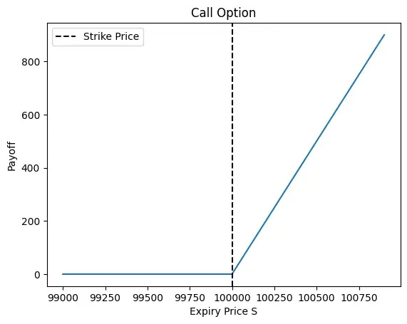
Table of Content
Payoff of an Option
Present Value
Option Price NOT equal Expected Payoff
Algebras, Filtrations and Martingales
Multi-period Binomial Model
American Options
Exotic Options
Multi-Asset Options
Final Remarks
Payoff of an Option
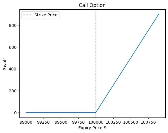
Let’s say you decide to buy a (european) BTC call with a strike price of $100k.
If BTC expires above $100k you would exercise your right to buy BTC at $100k and then immediately sell it for the spot price. Your payoff becomes S-K where S is the expiry price of the underlying and K is the strike price of the call.
If BTC expires below $100k you wouldn’t exercise your right to buy it at $100k since you can buy it for less so your payoff is simply 0.
Therefore for a call with strike price K the payoff is: max(S-K, 0)
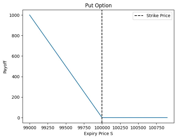
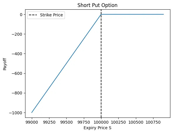
A put option gives you the right to sell the underlying at the strike price K so with the above logic the payoff becomes: max(K-S, 0)
Options are obviously not free so your total pnl will be: payoff - price of the option
As you can see with options you are limited to a loss of the price of the option and are not limited on how much you can make.
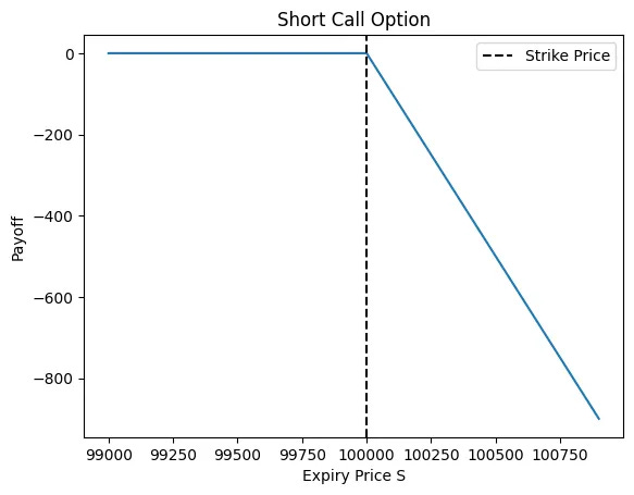
When selling an option this turns around, you earn at most the price of the option (that you receive immediately) but have unlimited downside.
Call writer payoff: min(K-S, 0)
Put writer payoff: min(S-K, 0)
Present Value
$100 in 1 month is not worth $100 right now. If you had $100 now you could invest in a risk-free asset with continuous yearly risk free rate r and you’d have e^(1/12 * r) * 100 in a month.
Doing this backwards you would have to invest e^(-1/12 * r) * 100 now to have $100 in a month.
So with yearly continuous interest of 3%, $100 in a month would be worth e^(-1/12 * 0.03) * $100 = $99.75 now.
This is called discounting back to present value and is important in pricing options since the payoff of an option lies in the future and we need to discount those payoffs back to know what those payoffs are worth NOW.
Besides continuous interest you can also use other forms of interest like discrete interest where you get paid every fixed amount of time like once a month or once a year.
With monthly discrete interest of 1%, $100 in a month would be worth (1 / (1 + 0.01)) * $100 = $99.01 now.
Option Price NOT equal Expected Payoff
Pricing an option is super easy then right? We just need to calculate the expected payoff of an option and discount that back and boom we have the options value now!
Unfortunately it’s not that simple.
We need to use this misunderstood and confusing concept called “risk-neutral probabilities” which are not really actual probabilities to begin with.
We can interpret them that way though because then the options profit does become the discounted expected payoff if you use those risk neutral probabilities for the expected values instead of the real-world probabilities.
They emerge from arbitrage-free valuation where we construct a portfolio that replicates the payoff of the option. Due to no-arbitrage the value of the option now has to be equal the value of the portfolio now because otherwise we could buy the cheaper and short the more expensive one and get an arbitrage profit since they have the same payoff.
Let’s consider the one-period binomial model as an example:
Assume the underlying price right now is $100 and it can either go up to $120 or go down to $80. Also assume we have a call option with a strike price K of $110.
If the underlying goes up our option will have a payoff of $10 and if it goes down then our option will have a payoff of $0.
We therefore want to construct a portfolio using the underlying and our bank account that’s worth $10 if the underlying goes up and $0 if the underlying goes down.
We buy/sell Delta of the underlying and have B in our bank account.
Assume that during the one period the risk-free rate / interest r is 0.01.
The bank account value after the one period (t=1) will then be (1+r) * B.
We get a system of equations:
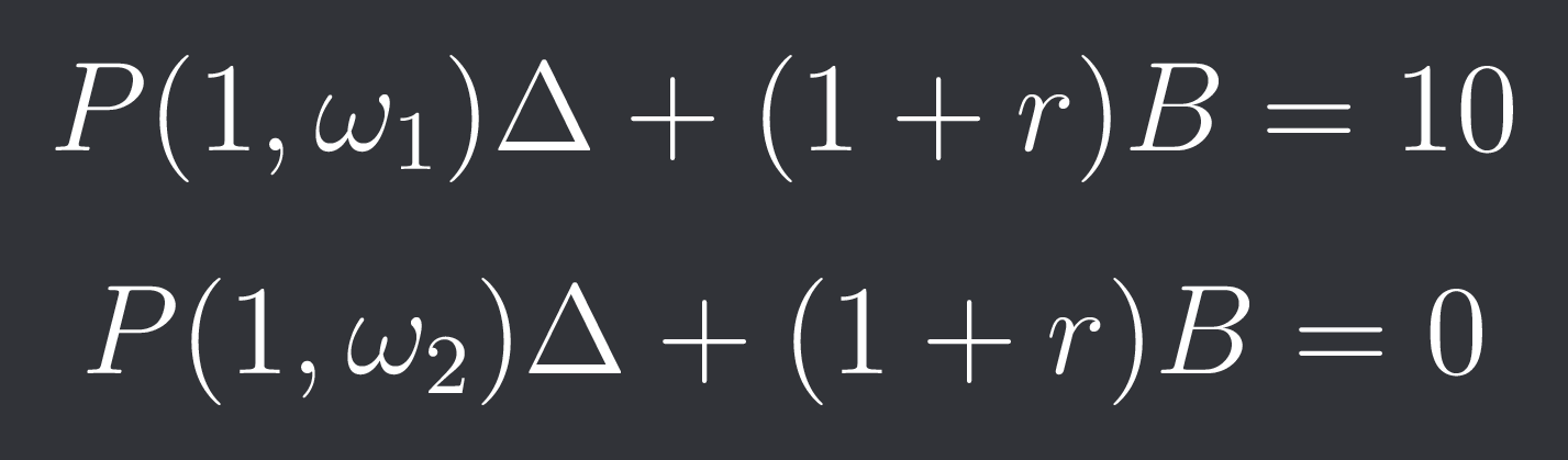
P(1, w1) is the price of the underlying at time t=1 in scenario 1 (up) and P(1, w2) is the price of the underlying in scenario 2 (down). So:
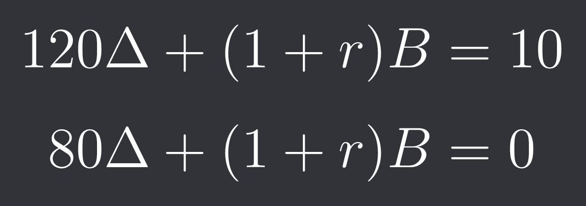
Subtracting equation 2 from equation 1 we get:

So Delta = 1/4.
Plugging this into equation 2 we get:
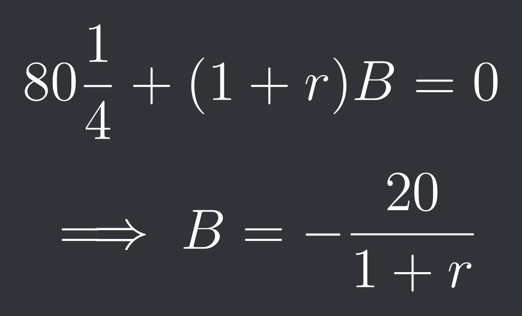
So we buy 1/4 of the underlying and borrow 20 / (1 + 0.01) = $19.80.
At time t=0 this has a value of:
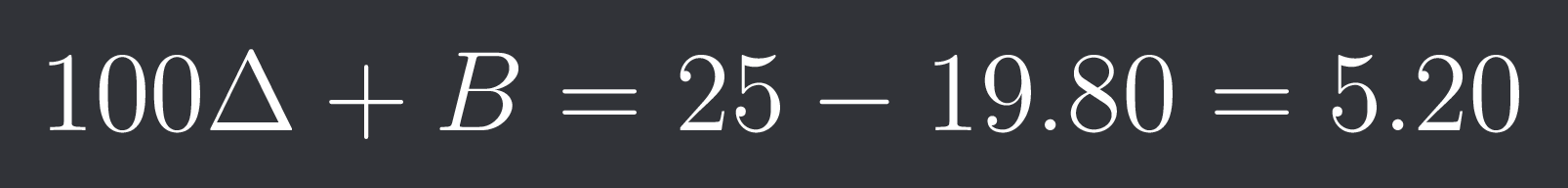
Since the option is worth the same as the portfolio the option is worth $5.20!
Note: The probability of price going up or down doesn’t matter in any of those equations. Intuitively you might have thought that if the probability of price going up was really high, say 99% then a call would become more expensive but that’s not the case!
This is the other method of pricing an option, finding a replicating / hedging portfolio for it and determining the value of the portfolio. Let’s use the risk-neutral probability approach now:
In a binomial model the risk-neutral probability of an up move is given by:

Where u is the relative up move (in our case 1.2) and d is the relative down move (in our case 0.8). I’m not gonna prove this here but you can do it yourself by setting up a portfolio of long underlyings and one short option and looking at the present value of the portfolio.
The risk neutral probability measure is then:
In our case q = 0.525.
The discounted expected payoff under risk neutral probability measure is then:
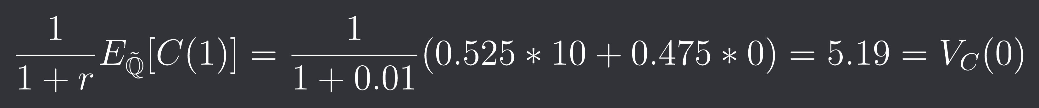
which (ignoring rounding errors) is the same result we got with the replicating portfolio! This is quite powerful as we can price any derivative we want now if we know its payoff. We simply need to calculate the expected value under risk-neutral probability and then discount back to present value.
Note: Risk-neutral probabilities are always positive and the expected value of the discounted price at time 1 under risk-neutral measure is equal to the price at time 0. We also have the equivalence:
There is no arbitrage
There exists a risk-neutral probability measure
We also have the equivalence:
Every derivative is attainable (we can find a hedging / replicating strategy for it). In this case we call the market complete.
There is exactly one risk-neutral probability measure
Algebras, Filtrations and Martingales
When going from one period to multiple periods we need to learn a little bit of math.
Assume we have K possible price paths. If we’ve already had some price movement we know that the true final price path we follow must be within a subset of the K price paths and that we cannot be within other price paths and can exclude them.
This is described by A_t. Assume there are 4 price paths Omega = {w1, w2, w3, w4}.
At time t=0 we could be within any price path so A_0 = Omega. At time t=T we’ve followed one price path exactly so A_T = {w1}, {w2}, {w3} or {w4}.
Here is an example: