Seasonality and Volatility Risk Premium

Coming up with market theories and creating new strategies

The previous article was an easy introduction to Market Making, we ran some simulations and built intuitive understanding for how market making actually performs in real markets.

In this article we are gonna look at a market seasonality and explain it’s outperformance.

If you end up enjoying this article consider getting the paid subscription, that way you can support me and I can write even more articles!
Here is a discount code for those interested: https://www.vertoxquant.com/eaf1ee4d

---

Table of Content

1. Seasonal Volatility

2. Forecasting Volatility via SAR

3. Volatility Risk Premium

4. Final Remarks

---

Seasonal Volatility

Volatility is not random, it has a couple of very clear seasonal effects. Let’s start with intraday volatility and build our way up.

I’m gonna be using data starting january 2018.

First let’s get the volatility by hour of day:

data = pd.read_csv("BTCUSDT-1h-data.csv")[["timestamp", "close"]].set_index('timestamp')
data.index = pd.to_datetime(data.index)

rets = data.pct_change(1).dropna()

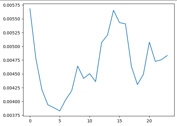
vol_arr = [np.mean(abs(ret)) for hour, ret in rets.groupby(rets.index.hour)]

So the we tend to get a lot of volatility around 2pm UTC and midnight UTC.
Let’s take a closer look using minutely data.

data = pd.read_csv("BTCUSDT-1m-data.csv")[["timestamp", "close"]].set_index('timestamp')
data.index = pd.to_datetime(data.index)

data['hour_minute'] = data.index.strftime('%H:%M')
data['rets'] = data['close'].pct_change(1).dropna()

data.dropna(inplace=True)

vol_arr = data.groupby('hour_minute')['rets'].apply(lambda x: x.abs().mean()).reset_index()

An interesting effect you can see is that volatility is very high at exactly midnight UTC and then very quickly drops off.
This can be explained by rebalancings, trades and whatever else happening automatically at midnight UTC.

You can also notice all those spikes with equal distance.
Those can be explained the same way.
Every time a “popular” candle like 15min, 30min, 1 hour, 4 hour closes you get a ton of volatility right at the close.

Now let’s look at the volatility by day of the week:

daily_data = pd.read_csv("BTCUSDT-1d-data.csv")[["timestamp", "close"]].set_index('timestamp')
daily_data.index = pd.to_datetime(daily_data.index)

daily_data['rets'] = daily_data['close'].pct_change(1).dropna()

daily_data.dropna(inplace=True)

vol_arr = [np.mean(abs(ret)) for dayofweek, ret in daily_data['rets'].groupby(daily_data.index.dayofweek)]

Here 0 stands for monday and 6 stands for sunday.
You can clearly see that weekends are less volatile than weekdays, this is because other financial markets are closed as well, there is less news, people aren’t working etc.

Now let’s get the vol by day of the month.

vol_arr = [np.std(ret) for day, ret in data['rets'].groupby(data.index.day)]

This is gonna be more noisy but looks like there is more vol in the middle of the month.

I wouldn’t put my hand in fire with this one though. The intraday and intraweek ones are the significant ones.

---

Forecasting Volatility via SAR

There are a ton of different volatility forecasting models like GARCH, HAR etc. but they all fail in one huge aspect. They don’t take into account seasonalities!
Most people just do an AR(1) forecast and then some additional transformations etc. like in GARCH.

We are gonna use a SAR model which stands for Seasonal Autoregressive model.
It extends the simple AR model by incorporating a seasonal term.

In practice you would use a more complex model like S-GARCH but that’s not the point of this article.

For volatility we are gonna use squared hourly returns.
Here is what that looks like:

data = pd.read_csv("BTCUSDT-1h-data.csv")['close']
data['rets'] = data.pct_change(-1)
data['vol'] = data['rets']**2

Now there are 2 approaches you can take.
You can do a regular AR(1) forecast and then adjust the prediction based on time of day and day of week OR you use 3 data points in your forecast, the vol 1 hour ago, the vol 24 hours ago and the vol 168 hours (1 week) ago.

I’m gonna use version 2 as it’s a lot more practical.

We can easily estimate the coefficients with multiple regression.

This seasonality is even more extreme with fees and gas. You can predict those very accurately with the simple model above.

---

Volatility Risk Premium

Now since more volatility markets are more risky (risk measured in volatility) we would expect to get more return if we are exposed to higher volatility.

This is called a risk premium, additional return for additional risk.
Let’s plot the average return by hour of day and average vol by hour of day next to each other.

vol_arr = [np.mean(abs(ret)) for hour, ret in rets.groupby(rets.index.hour)]
ret_arr = [np.mean(ret) for hour, ret in rets.groupby(rets.index.hour)]

Looks like our theory is right for the most significant one! If we hold from midnigh to 1am UTC we get a ton of volatility but also a positive return. After that the volatility quickly drops off and our returns become negative.

Let’s try and trade this both ways.
We will buy BTC at midnight UTC and sell at 1am UTC.
We will short BTC at 1am UTC and buy back at 3am UTC.

That looks fantastic buuut don’t get your hopes up. Fees will destroy you with a strategy like this. You could try and execute via limit orders though, just not with taker.

Now let’s use the same logic for day of week:

vol_arr = [np.mean(abs(ret)) for dayofweek, ret in data['rets'].groupby(data.index.dayofweek)]
ret_arr = [np.mean(ret) for dayofweek, ret in data['rets'].groupby(data.index.dayofweek)]

A lot more noisy but there could still be some effect.
With this one you would theoretically be long during the weekdays but the effect is not significant enough.

---

Final Remarks

In this article we came up with some theory for a market effect and were able to succesfully use it to our advantage!
This should be your goal with everything you do in quant imo.
I’m not a fan of the data mining approach where some random signal shows up among random numbers and magically works. Everything should make sense economically.