
Why Mean-Variance Optimization Breaks Down
And how to make it actually work

Introduction
Mean–Variance Optimization (MVO) is a central framework for portfolio construction: choose weights that balance expected return against risk as measured by variance.
In its classical form, MVO is elegant, convex (under mild conditions), and analytically tractable. Yet practitioners quickly encounter a paradox: the mathematically “optimal” portfolio built from estimated inputs is often unstable, highly leveraged (explicitly or implicitly), and disappoints out-of-sample.
This is not a minor implementation detail; it is a structural consequence of combining a high-dimensional optimizer with noisy estimates of expected returns and covariances.
This article develops MVO from first principles and then explains, in a mathematically explicit way, why raw MVO tends to maximize estimation error.
Finally, it surveys the spectrum of practical fixes, organized around two levers: (i) improving or regularizing the inputs (expected returns and covariances), and (ii) constraining or regularizing the optimizer (the feasible set and the objective).
The unifying theme is that almost every successful “fix” works by injecting bias in exchange for a large reduction in variance of the resulting portfolio weights, thereby improving out-of-sample performance and implementability.
The Classical Framework
Notation
Consider N risky assets. Let the random vector of (excess) returns over a single period be
Define the (unknown) population mean and covariance
A portfolio is a weight vector interpreted as a fraction of capital invested in each asset.
The basic budget constraint is
where 1 denotes the all-ones vector in R^N. In other words, the weights should sum up to 1. Additional constraints like no-short, leverage limits, or sector bounds will be presented in the following chapters.
Under this setup, the portfolio return is linear in weights:
The expected portfolio return and variance are
Two foundational facts are worth stating explicitly because they explain why MVO becomes a quadratic program:
1. Expected return is linear in weights. This makes the “reward” side easy to compute but also extremely sensitive to errors in mu, because the optimizer can exploit tiny differences in mu via large weight changes.
2. Variance is quadratic in weights. The covariance matrix Sigma couples assets through correlations: diversification is precisely the exploitation of off-diagonal terms in Sigma. The quadratic form w^T Sigma w is convex in w if Sigma is positive semidefinite, and strictly convex if Sigma is positive definite, which ensures the uniqueness of the minimum-variance solution under typical linear constraints.
The Markowitz Problem in Matrix Form
Markowitz’s original formulation can be stated as: among all portfolios with a given expected return, choose the one with minimum variance. Fix a target expected return m. The constrained optimization is
If short-selling is disallowed, one adds w >= 0 componentwise. If leverage is limited, one might add |w|_1 <= L, where |.| denotes the L1 norm, and so on.
Why is the covariance matrix central here? Because for any two assets i and j,
The diagonal terms w_i^2 Sigma_{ii} represent contributions from each asset’s variance; the off-diagonal terms w_i w_j Sigma_{ij} represent interaction through co-movement. Diversification is not “holding many assets” per se; it is selecting weights so that positive and negative interactions among returns reduce overall variance.
A subtle but important point: variance is a second-moment object. It treats positive and negative deviations symmetrically and is fully described by Sigma. This makes MVO analytically convenient, but it also means the framework inherits all limitations of second-moment risk measures; non-normality, fat tails, and asymmetry are not captured unless the distribution is (approximately) elliptical. In many institutional contexts, however, variance remains a useful proxy because it aligns with tracking error, volatility targets, and risk budgeting infrastructure.
The penalized (risk-aversion) form and its equivalence
An equivalent way to pose the trade-off is to maximize a mean-variance utility function:
where gamma > 0 is the risk-aversion parameter. Larger gamma penalized variance more heavily, shifting the solution toward lower-risk portfolios.
The equivalence between (MVO-1) and (MVO-2) is practically important. The constrained form (MVO-1) traces the efficient frontier by varying m. The penalized form (MVO-2) traces it by varying gamma. In many production systems, gamma is tuned to meet a risk target or tracking error budget.
Solving the classical problem: Lagrangian and closed-form structure
To make mechanics concrete, consider (MVO-2) without additional constraints beyond the budget constraint. Form the Lagrangian
with Lagrange multiplier eta enforcing 1^T w = 1.
First-order optimality (assuming Sigma is positive definite) gives
hence
Imposing the budget constraint 1^T w = 1 yields
so
Substituting (1.2) into (1.1) gives the explicit optimizer.
This expression reveals a key structural fact that will matter later: the optimal weights are built from Sigma^{-1} mu and Sigma^{-1} 1. In other words, the inverse covariance matrix is the central operator transforming expected returns into weights. When Sigma^{-1} is unstable (ill-conditioned or poorly estimated), the entire solution becomes unstable.
For the return-target form (MVO-1), the Lagrangian with multiplies lambda, eta is
The first-order condition is
Define the classical scalars
Assuming Sigma is positive definite and mu is not collinear with 1 under Sigma^{-1}, one has Delta > 0. Solving for lambda, eta yields a closed-form frontier, and the efficient frontier in (sigma^2, m) space is a parabola:
The frontier’s curvature and location are completely determined by (A,B,C), i.e., by Sigma^{-1} and mu. This already hints at the practical challenge: every point on the frontier depends on inverting Sigma and multiplying by mu, precisely the operations most vulnerable to estimation noise.
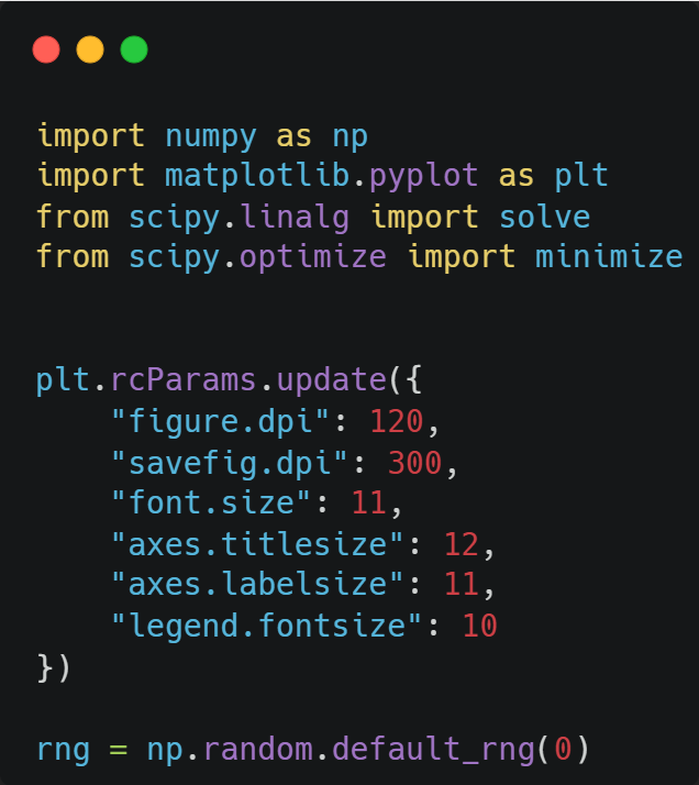
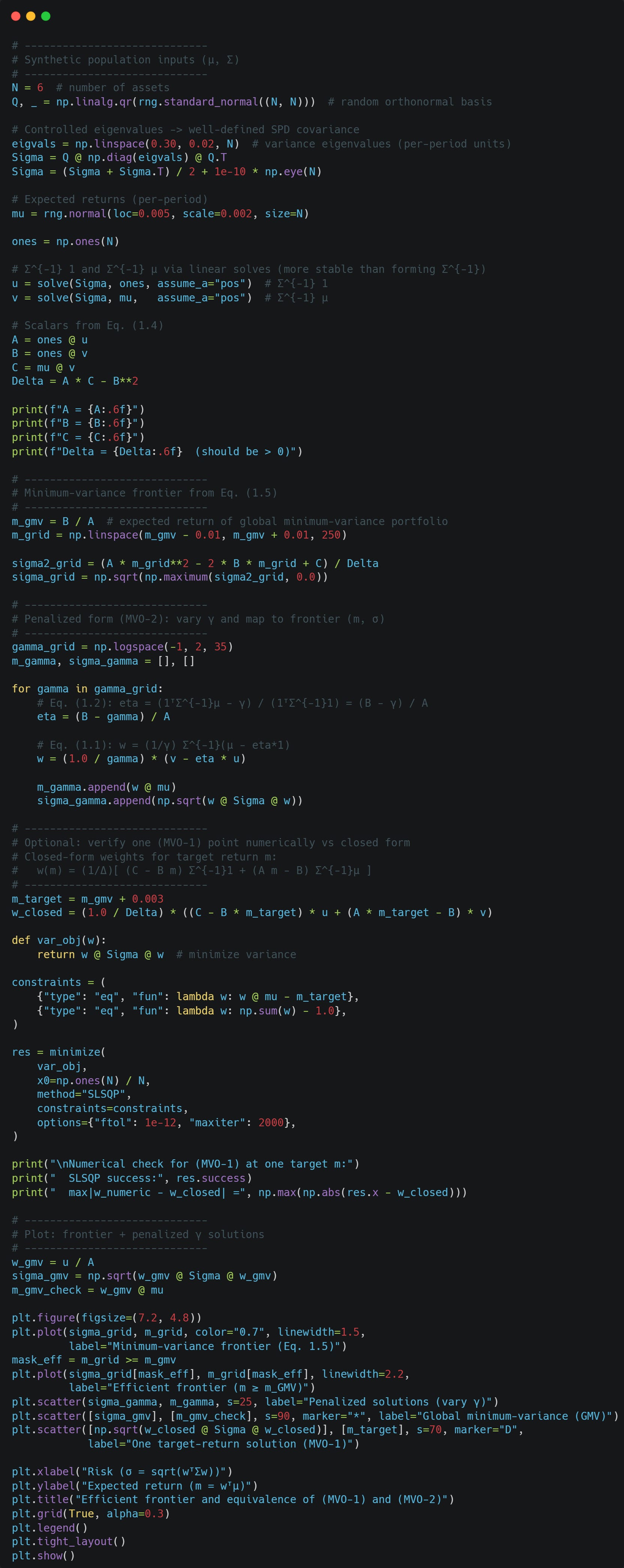
Let’s implement this in Python and look at the resulting efficient frontier. We will also compare our closed-form solution of (MVO-1) to a numerical solution to verify that we did everything right.
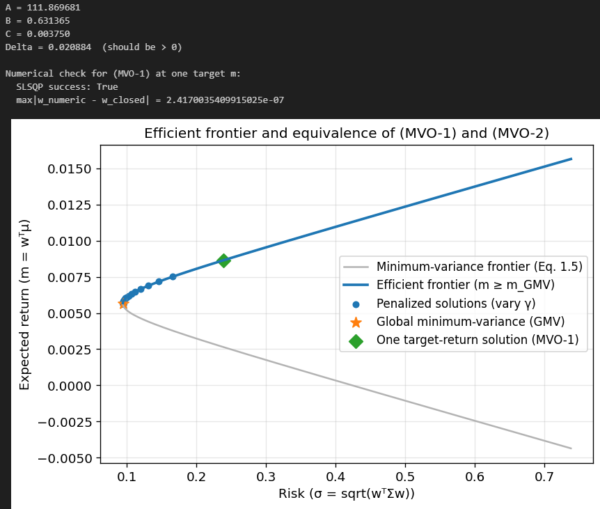
As you can see, our closed-form solution and numerical solution are pretty much identical, and the (MVO-2) solutions lie on the efficient frontier traced by the (MVO-1) solution, so they are indeed equivalent.
Interpreting Sigma: Risk Geometry and Diversification
It is useful to interpret the quadratic form geometrically. If Sigma is positive definite, then the set of portfolios with equal variance sigma^2,
is an ellipsoid in weight space. The optimizer in (MVO-2) chooses the point on the budget hyperplane {1^T w = 1} that maximizes a linear functional w^T mu minus a quadratic penalty. The optimum balances moving “up” in the direction of mu while staying within low-risk ellipsoids determined by Sigma.
This picture is clean when mu and Sigma are known. The moment we replace them with estimates, the ellipsoids tilt and stretch unpredictably, and the direction of “up” becomes noisy. The optimizer, being deterministic, will still choose an extreme point, often an extreme point of the wrong geometry. That is the beginning of the “error maximization” story.
Here is an example using two assets:
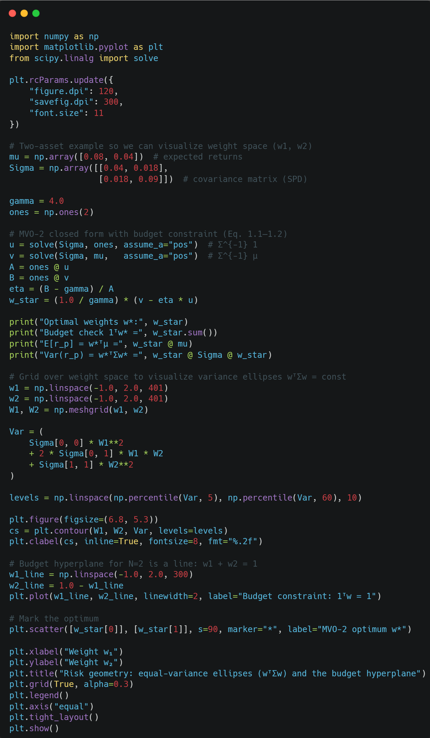
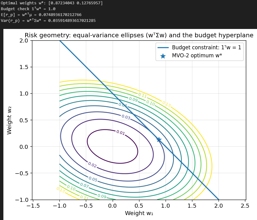
Each ellipse here corresponds to portfolios with equal variance. As you can see, our optimal portfolio just barely touches the 0.03 variance ellipsoid, and any other portfolio on the line (that satisfies the budget constraint) results in a higher variance.
The “Error Maximization” Problem
Raw MVO is often described informally as “garbage in, garbage out.” That statement is true, but it understates the severity: MVO does not merely propagate input error; it can amplify it. In high dimensions, the amplification can be dramatic enough that the optimizer effectively learns the noise in the estimated inputs.
This section makes that mechanism explicit.
MVO is not an optimization problem; it is a statistical decision problem
In theory, (mu, Sigma) are population quantities. In practice, we never observe mu or Sigma. We observe a finite time series
and produce estimators hat{mu} and hat{Sigma}. The most common “plug-in” estimators are the sample mean and covariance
Then the raw MVO portfolio is
or its return-target equivalent.
Crucially, hat{w} is a function of the random sample; it is itself random. The “true” objective we actually care about is out-of-sample performance under the true distribution, e.g., maximizing
But plug-in MVO maximizes a different random objective,
The practical question is not “is hat{w} optimal for hat{U}?” (it is, by construction), but “how does U(hat{w}) compare to U(w^\star), where w^\star maximizes U?” That gap is the cost of estimation error and model uncertainty.
Why expected return estimation is the Achilles’ heel
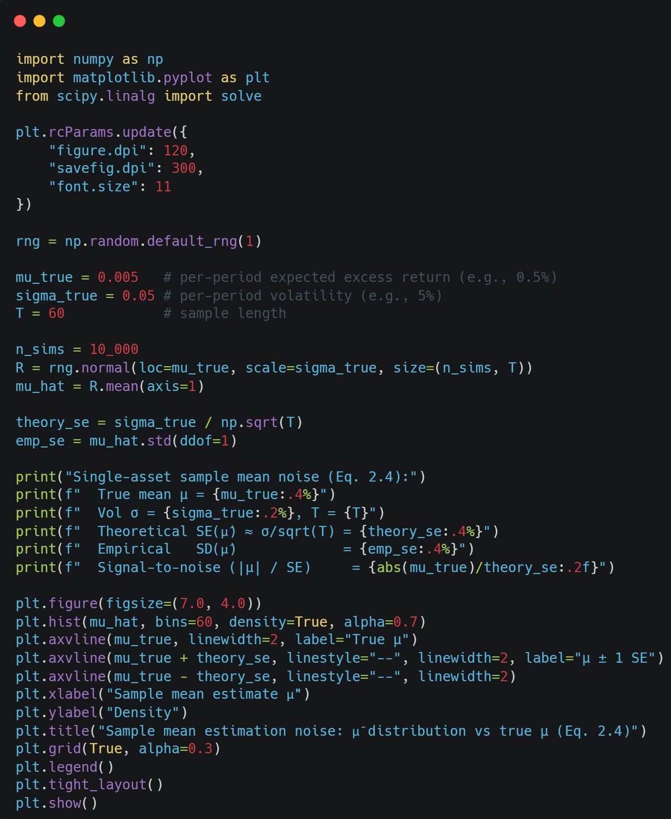
Start with expected returns. For each asset i, the sample mean hat{mu}_i has a standard error on the order of
where
In many liquid asset classes, annualized volatilities might be 10% - 30% while annualized expected excess returns might be 2% - 8%. Translating to a monthly scale, the noise in the sample mean can be comparable to, or larger than, the signal. This is a fundamental signal-to-noise limitation, not an implementation defect.
Now multiply that limitation by dimensionality. MVO compares assets and tries to exploit differences in mu. When mu is noisy, the differences the optimizer sees are often dominated by noise. The optimizer is then rewarded (in-sample) for taking large positions in the assets that happened to have high realized returns in the estimation window, even if that was random luck.
Because the expected return term w^T mu is linear, any error in mu shifts the gradient of the objective directly. In contrast, the covariance term is quadratic and tends to act as a smoothness penalty. This asymmetry is why MVO is particularly fragile to errors in mu.
Here is a simple numerical simulation of how much noise can affect our estimate of mu:
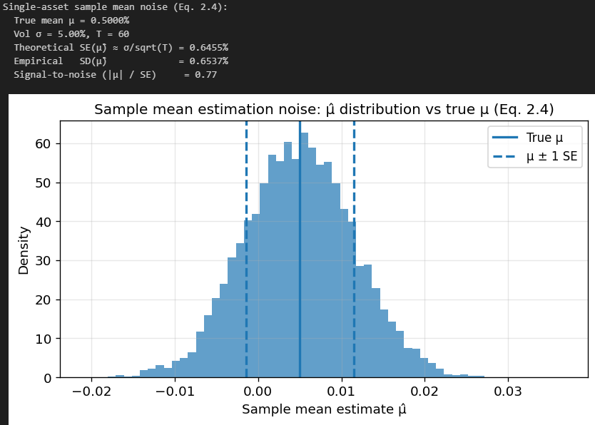
And now the impact on our portfolio weights from MVO. We assume 20 assets with identical true means, so any variation in mu is pure noise.
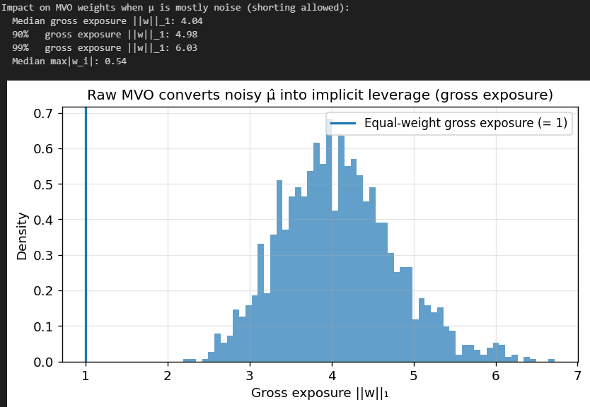
Our gross exposure is through the roof! A typical MVO portfolio here is equivalent to 200% long and 200% short, 4x leverage. Our right tail on Gross Exposure is also huge, so the portfolio sometimes ends up being 6x levered. The largest single position is also 54% of the portfolio, even though we have 20 assets.
This shows just how much of an extreme impact estimation noise in mu has on MVO.
Why covariance estimation becomes dangerous when inverted
The second failure mode is subtler: even if covariance estimates are “more stable” than mean estimates, the optimizer requires hat{Sigma}^{-1}. Inversion is the mathematical operation that turns moderate estimation noise into potentially huge weight noise.
To see why, consider the eigen-decomposition of the true covariance matrix:
where Q is orthonormal and
with lambda_i > 0$ if Sigma is positive definite. Then
Small eigenvalues become large eigenvalues after inversion. In portfolio terms, eigenvectors associated with small variance directions are precisely the directions the optimizer finds attractive: they offer “cheap risk.” But in finite samples, the smallest eigenvalues of hat{Sigma} are often dominated by noise (especially when T is not much larger than N). When the optimizer leans on these noisy low-variance directions, it produces extreme, unstable weights.
This is not hypothetical. A basic dimensionality fact already creates a hard boundary: if T < N, the sample covariance hat{Sigma} is singular (rank at most T-1), so hat{Sigma}^{-1} does not exist. Even if T is only moderately larger than N, hat{Sigma} can be ill-conditioned, making numerical inversion unstable and conceptually unreliable.
Let’s consider three cases: T < N, T ≈ N, and T > N, and look at the impact that T has on the estimated eigenvalues:
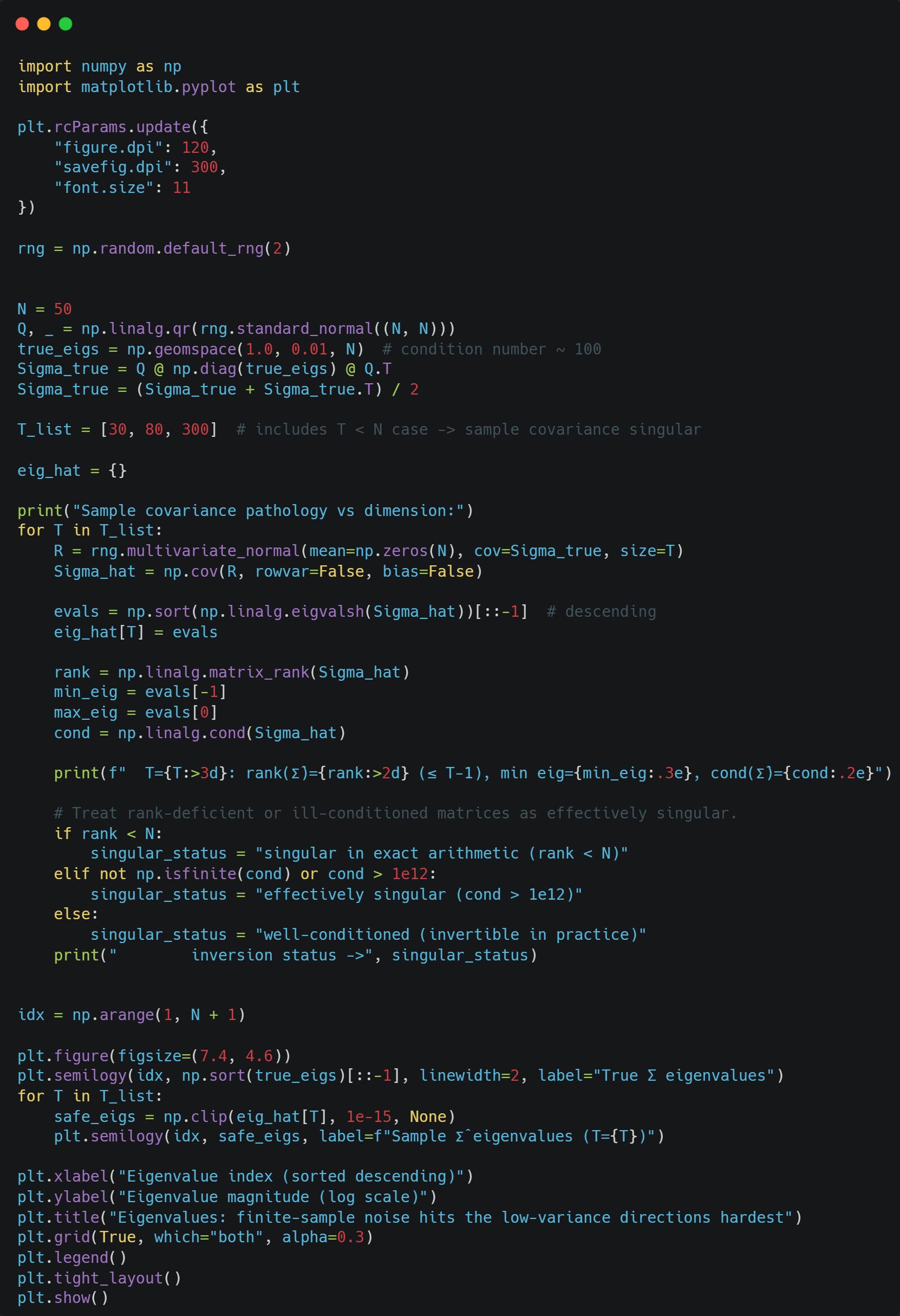
You can clearly see one thing: For the estimates where T = 30, Sigma becomes singular, and the 30th and further smallest eigenvalues just become 0. For T = 80, we can still see that the smaller eigenvalues are systematically underestimated. The estimates become better as we increase T to 300.
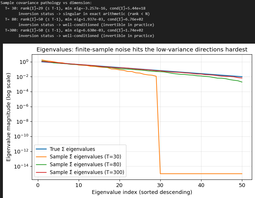
Now, let’s look at estiamted eigenvalues of Sigma and Sigma^{-1} for T=300:
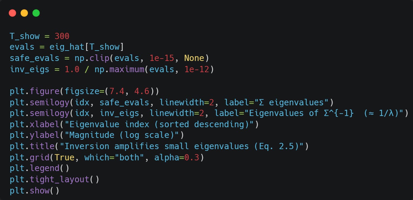
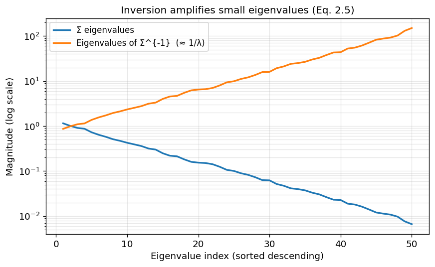
The smaller the estimated eigenvalues, the larger the estimated eigenvalues of the inverse of Sigma.
Note: The y-axis is logarithmic on both plots, so linear → exponential!
Sensitivity Analysis: How estimation errors translate into weight errors
A useful way to formalize “error maximization” is to compute how small perturbations in mu and Sigma affect the optimizer.
Consider the unconstrained (besides budget) mean–variance utility maximization (MVO-2). The population optimum satisfies
with eta^\star chosen to enforce 1^T w^\star = 1. The plug-in estimate is
Write estimation errors as
A first-order expansion (informally, a matrix Taylor approximation) uses
A first-order perturbation of the optimizer gives
The last term enforces the budget constraint (with delta eta the perturbation in the multiplier); dropping it isolates the two main channels.
Several qualitative conclusions drop out of (2.8):
1. Mean error passes through Sigma^{-1}. Even if delta mu is moderate, multiplying by Sigma^{-1} can produce large changes in w, especially in directions corresponding to small eigenvalues of Sigma (or hat{Sigma}).
2. Covariance error enters as a “sandwich” with Sigma^{-1}. The term Sigma^{-1} * delta Sigma, w^\star has Sigma^{-1} on the left; if w^\star already has large exposures along unstable directions, covariance errors further distort them.
3. Budget adjustment can amplify instability. The multiplier eta is computed using 1^T Sigma^{-1} mu and 1^T \Sigma^{-1} 1$. If either of these scalars is unstable due to \Sigma^{-1}, the adjustment needed to enforce 1^T w=1 can itself swing drastically.
The key is not that delta mu and delta Sigma exist—of course they do—but that MVO transforms them with Sigma^{-1}, a potentially high-gain operator.
Let’s see how a badly conditioned Sigma affects delta w. We’ll drop the budget constraint so eta doesn’t influence the analysis:
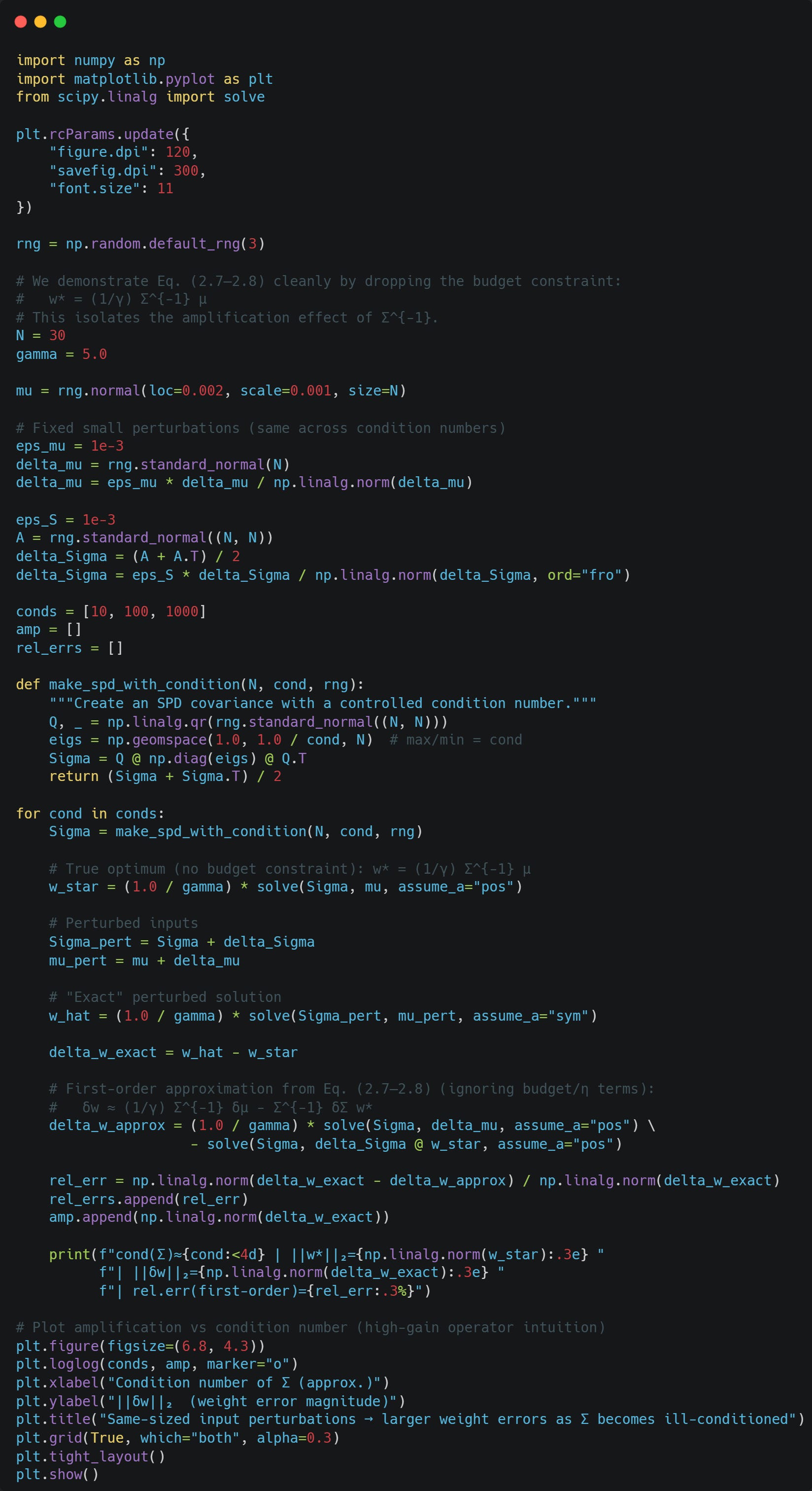
You can see clearly that as Sigma becomes ill-conditioned, the error in w grows.
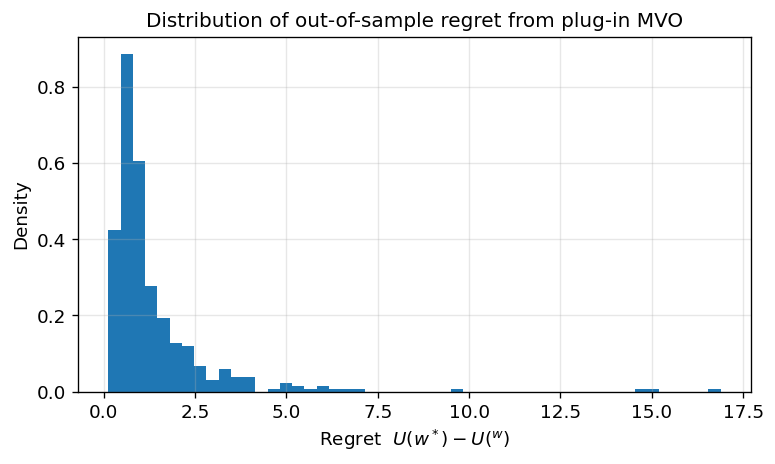
Optimizer’s curse
Another lens is the optimizer’s curse, a general phenomenon in statistical decision-making: if you choose the argmax of a noisy objective, the achieved value is biased upward in-sample, and the chosen decision is biased toward noise.
Formally, because hat{w} maximizes hat{U}(w),
but what matters is U(hat{w}). The difference
is typically positive and can be large in high dimensions. Intuitively, among many portfolios, some will look exceptionally good in-sample purely due to noise in hat{mu} and hat{Sigma}. MVO systematically selects those portfolios and then “locks in” their noisy characteristics via extreme weights.
This selection effect is strongest when:
The number of assets N is large relative to the sample size T
Expected return estimates are weak (low signal-to-noise);
Shorting/leverage is permitted (large feasible set);
Constraints are loose (optimizer can chase small estimated edges);
The covariance matrix has near-collinear assets (ill-conditioning).
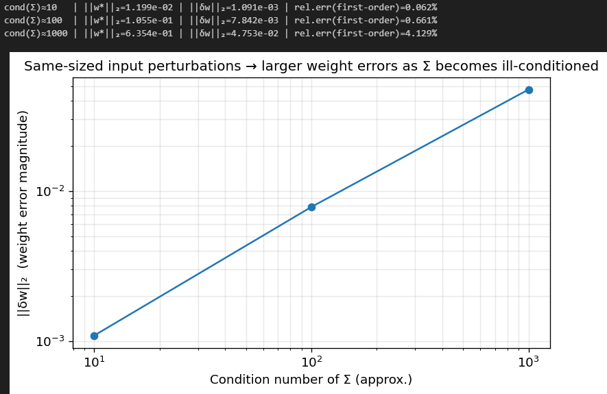
Let’s demonstrate the optimizer’s curse via Monte-Carlo.
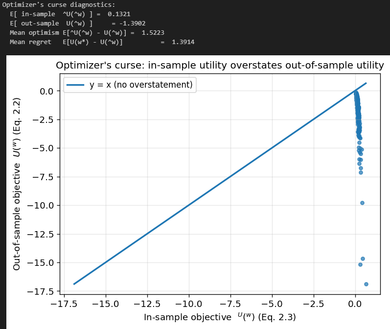
You can see that even in an environment with equal true in- and out-of-sample mu and Sigma, due to estimation error, we vastly overestimate our utility in the in-sample.
Practical Symptoms: Instability, extreme positions, turnover, and disappointment
When raw MVO meets real data, the mathematical mechanisms above manifest in operational ways:
Extreme weights and implicit leverage. Even with the budget constraint 1^T w = 1, weights can be large positive and large negative (if shorting is allowed), producing large gross exposure |w|_1. Even with no-short constraints, solutions often sit on corners of the feasible region (many weights at bounds), because linear return objectives push to extremes.
High sensitivity to small input changes. Updating the estimation window by one month can materially change hat{mu} and hat{Sigma}, leading to large changes in hat{w}. This is not merely “rebalancing”; it is model instability.
High turnover and transaction cost drag. If weights change drastically, realized performance is dominated by trading costs and market impact, neither of which exists in the clean Markowitz formulation unless explicitly modeled.
Out-of-sample underperformance relative to naive allocations. A simple equal-weight or risk-parity portfolio can outperform a naive MVO portfolio after costs, not because those heuristics are theoretically superior, but because they are robust to estimation error.
These observations motivate the central practical conclusion: raw plug-in MVO is a high-variance estimator of portfolio weights. In modern terms, it is an overfit model.
The Spectrum of Solutions
This concludes the theoretical foundation.
The remaining 40 pages implement and test 11 robust portfolio construction techniques.
Each technique includes: Mathematical derivation → Clean implementation → Parameter tuning → Comparative results
Plus: Full research notebook (1250+ lines) with production-ready code. If you've made it this far through the theory, the implementations are where it pays off.
If raw MVO is fragile because it optimizes a noisy objective with unstable operators, then fixes must do one (or both) of the following:
1. Fix the inputs: replace (hat{mu}, hat{Sigma}) with estimators that have lower estimation error, better conditioning, or an economically grounded structure.
2. Constrain or regularize the optimizer: modify the optimization problem so that it cannot translate small input errors into extreme weight changes.
These approaches are complementary. Many production-grade systems use both: structured/shrunk inputs and a constrained, regularized optimization.
Fixing the inputs
Covariance Shrinkage: Stabilizing \hat{Sigma} and its inverse
The sample covariance hat{Sigma} is unbiased under idealized assumptions, but it can have high variance in finite samples, especially for off-diagonal elements. Shrinkage addresses this by pulling the estimate toward a structured target F that is lower variance but potentially biased.
A canonical shrinkage estimator is
Common choices for F include:
a diagonal matrix (imposing zero correlations),
a constant-correlation model,
a factor-based covariance (discussed next),
an identity-scaled matrix (equal variance, no correlation).
Why does shrinkage help? Because it increases the smallest eigenvalues of hat{Sigma} (or, more precisely, it reduces eigenvalue dispersion), improving the condition number and stabilizing inversion. In terms of Sigma^{-1} mu, shrinkage reduces the optimizer’s ability to exploit noisy “cheap-risk” directions created by small sample eigenvalues.
A useful way to view this is that shrinkage imposes a prior belief: extreme correlation structures are unlikely unless supported by strong data. By nudging the estimate toward a simpler structure, you reduce estimation variance more than you increase bias, improving out-of-sample performance.
Oracle note: In the sweep below, the “best delta” is chosen by maximizing utility computed with the true (mu, Sigma) to isolate the mechanism. In practice, delta must be selected via an analytic estimator (e.g., Ledoit–Wolf/OAS) or via walk-forward / nested cross-validation. We also report a held-out test-sample utility proxy for evaluation, not for selection.
Let’s look at the effect of choosing different values of delta. We will let F be
which has the average estimated variance among all assets as its diagonal entries.
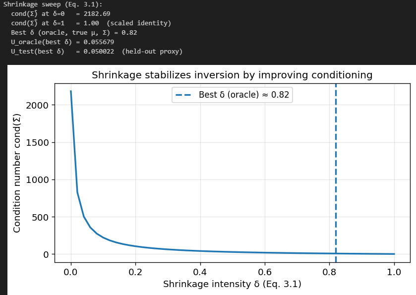
As you can see, the condition number of our estimated covariance matrix reduces pretty greatly as we increase delta.
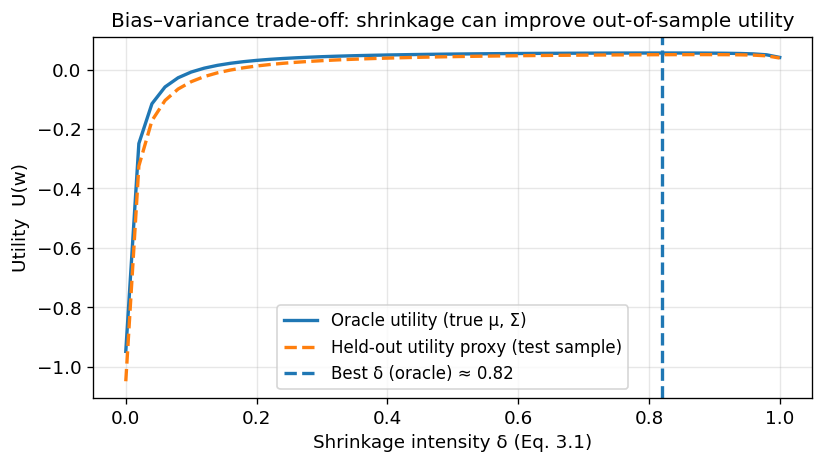
Utility increases out of sample as we increase delta (This is what we REALLY care about!)
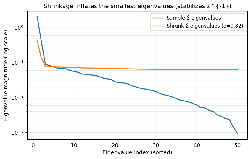
Small eigenvalues are inflated instead of dropping to extremely low values, which in turn causes the eigenvalues of Sigma^{-1} to not explode.
Factor Models
A deeper way to control covariance noise is to assume returns are driven by a small number of common factors. A standard linear factor model is
where
f in R^K are factor returns with K << N
B in R^{N x K} are factor loadings
epsilon in R^N are idiosyncratic returns.
Assuming epsilon is uncorrelated with f and has diagonal covariance D, the covariance of r becomes
where Sigma_f = Cov(f) and D = Cov(epsilon) is typically diagonal.
The parameter-count reduction is dramatic. A full covariance matrix has N(N+1)/2 unique parameters. A factor model estimates:
NK loadings (often constrained/regularized)
K(K+1)/2 factor covariances
N idiosyncratic variances.
When K << N, this is a much lower-dimensional estimation problem, leading to more stable covariance estimates and more stable inverses. Economically, factors capture persistent co-movement structure (industries, styles, macro exposures), while idiosyncratic risk captures asset-specific variance.
For optimization, (3.3) has another advantage: it makes risk decomposition interpretable and enables direct factor exposure constraints, a major practical tool for controlling unintended bets.
To test this method, we are gonna assume assets follow some “true” factor model, and then we will estimate this factor model to obtain an estimate for Sigma by plugging the estimates into (3.3):
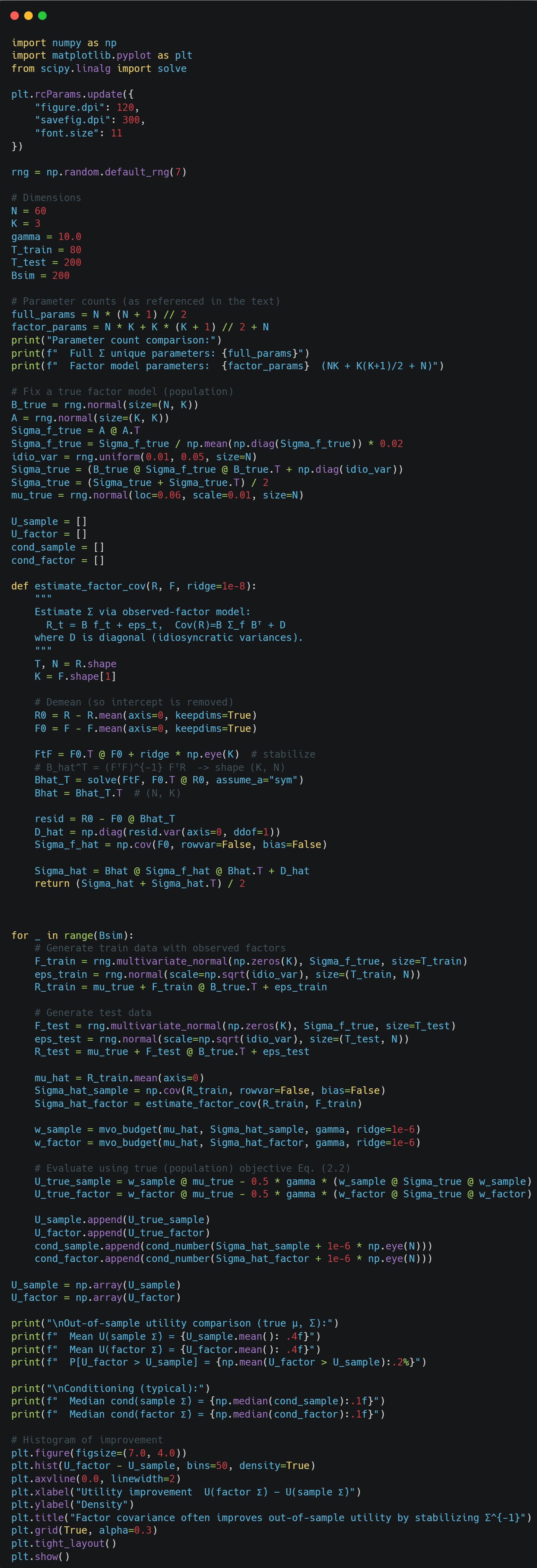
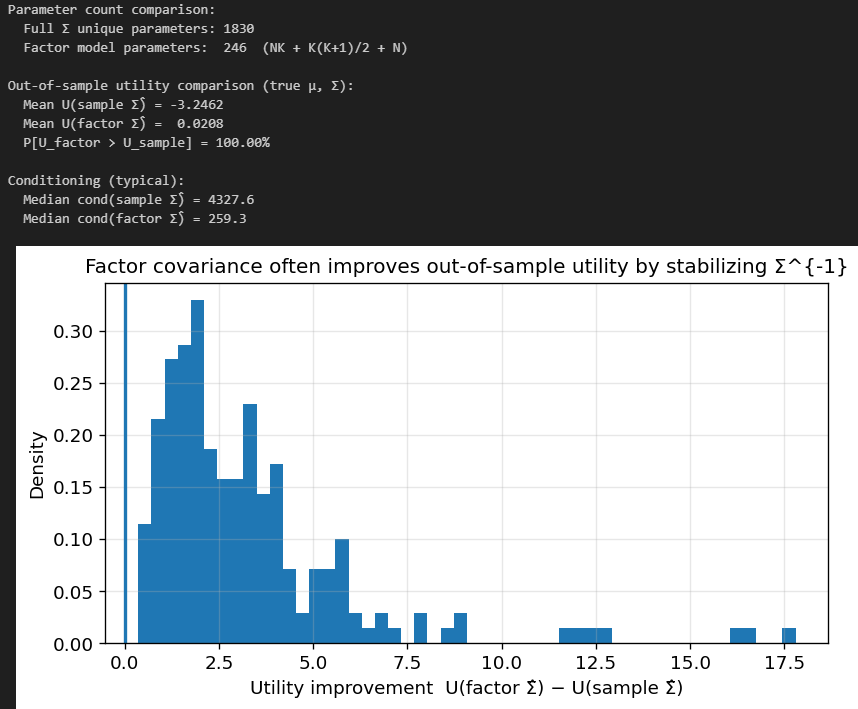
As you can see, our median condition went from 4327 for the naive sample covariance to only 259.3 for the factor-informed covariance. Utility improved 100% of the time out of sample!
Time-varying covariance
Covariances evolve over time. Using very long histories can reduce sampling error but introduce model error if the distribution is non-stationary. Using short histories reduces model error but increases estimation noise.
A common compromise is an exponentially weighted covariance estimator. For a finite window, a normalized form is
This places more weight on recent observations, adapting to changing regimes, while keeping the weights normalized for finite T.
An equivalent way to write the estimator is the recursive form
which implicitly normalizes and becomes equivalent to the sum as T → infinity (since lambda^T → 0).
But note: exponential weighting alone does not solve ill-conditioning in high dimensions; it is often combined with shrinkage or factor models.
The practical point is that “better covariance” means balancing estimation variance against non-stationarity. MVO fails when either error dominates, and real markets usually give you both.
Expected Returns
If covariance estimation is difficult, expected return estimation is usually worse. Many practical systems, therefore, treat mu not as a directly estimated sample mean, but as a forecast that must be heavily regularized.
A basic shrinkage approach is
where mu_0 is a prior mean. Choices for mu_0 include:
zero (implying no predictability in excess returns),
a cross-sectional average (implying mean reversion across assets),
factor-model-implied returns,
equilibrium-implied returns from a benchmark portfolio.
The key is the logic: because hat{mu} is high-variance, we deliberately introduce bias by shrinking toward a stable prior. This reduces the variance of the resulting weights, which is often the dominant out-of-sample benefit.
A particularly influential equilibrium anchoring method is to infer implied expected returns pi from an observed “market” or benchmark portfolio w_m.
Before invoking the next equation, it helps to distinguish between two regimes:
Risk-free asset (tangency portfolio). If a risk-free asset is available and w_m is the tangency portfolio, then pi are excess returns and reverse optimization yields pi = lambda Sigma w_m.
Risky-only, fully invested. If we remain in the 1^T w = 1 setting, the KKT condition is mu = gamma Sigma w_m + eta 1. The intercept term is economically irrelevant under the budget constraint, so one can normalize it away or interpret eta as the baseline rate.
In a mean–variance world, if w_m is optimal for some representative investor with risk aversion lambda, then
This produces a return vector pi consistent with the covariance structure and observed holdings. Even if the exact assumptions are stylized, pi has a crucial practical advantage: it is anchored to a diversified, implementable portfolio, which prevents the optimizer from forming extreme views unsupported by the market’s aggregate positioning.
Black-Litterman as a canonical “fix-the-inputs” framework
Black–Litterman formalizes the idea that expected returns should be a blend of (i) equilibrium returns and (ii) investor views. While many variants exist, the classical setup can be summarized as follows.
Let pi be equilibrium implied returns (e.g., from (3.6)). Model the prior as
where tau > 0 scales uncertainty in the prior. Investor views are expressed as
where P in R^{M x N} selects linear combinations of returns, q in R^M are view returns, and view noise has covariance Omega in R^{M x M}$ (often diagonal).
The posterior mean under Gaussian assumptions is
Why does this help MVO?
It shrinks noisy, unconstrained return estimates toward an equilibrium anchor.
It expresses uncertainty explicitly via tau and Omega, preventing overconfidence.
It ensures that when views are weak or absent, the optimizer defaults to a diversified baseline rather than a noisy corner solution.
Black–Litterman is not magic; it is a disciplined way of injecting structure and uncertainty into mu, which is exactly what raw MVO lacks.
Resampling and Bayesian Averaging: Stabilizing weights instead of moments
Another approach is to accept that inputs are noisy and average over that uncertainty. A simple version is bootstrap resampling:
1. Generate many synthetic datasets by resampling {r_t}.
2. For each dataset b, compute hat{mu}^(b), hat{Sigma}^(b) and solve MVO to get hat{w}^(b).
3. Average weights:
The intuition is that extreme positions caused by noise tend not to be stable across resamples; averaging dampens them. In decision-theoretic language, this approximates integrating over parameter uncertainty rather than conditioning on a single plug-in estimate.
This class of methods “fixes” MVO not by producing perfect estimates, but by reducing the variance of the decision w.
Let’s compare the weights generated by this method with those of MVO using just the sample estimates. We will also enforce long only to make the weights more comparable.
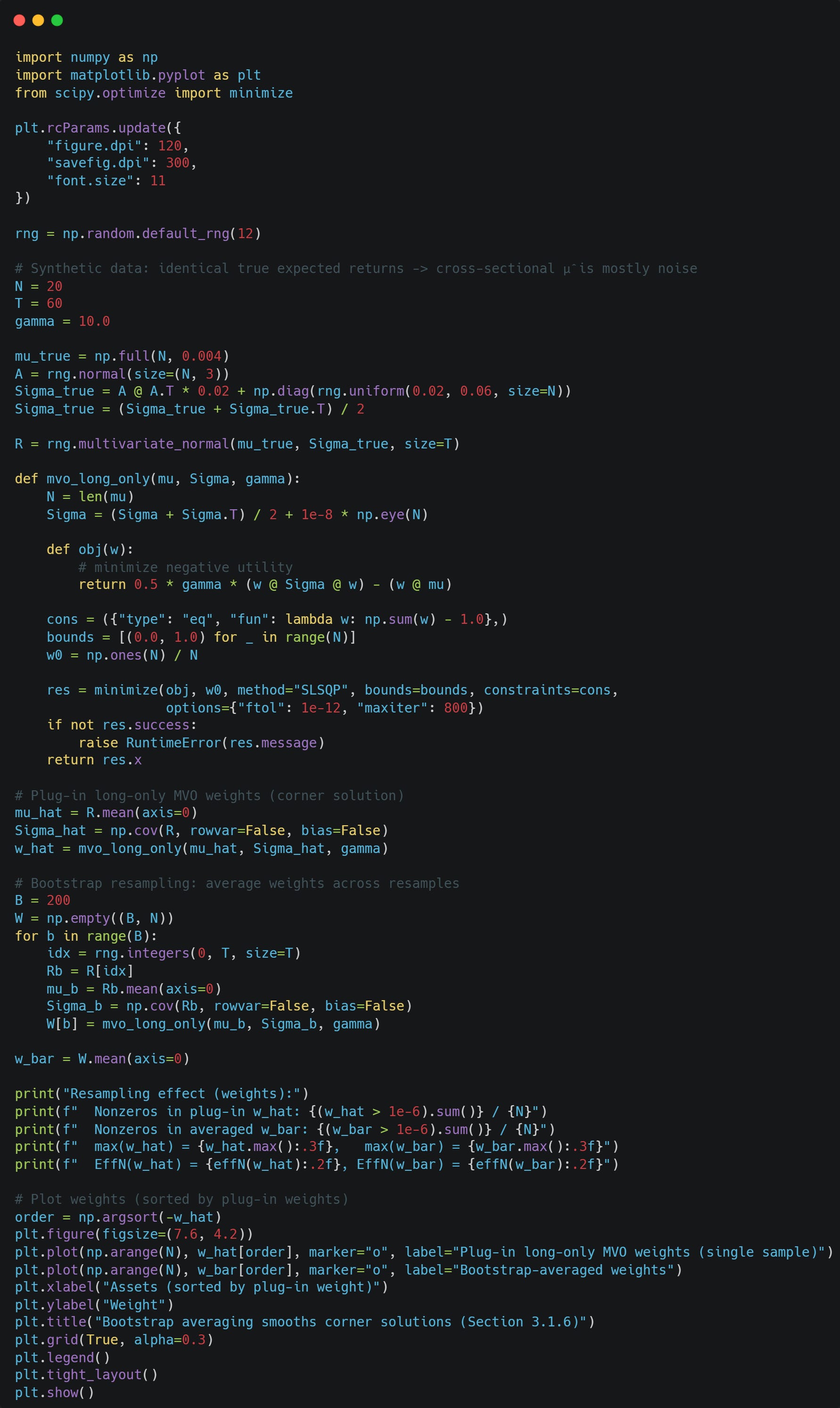
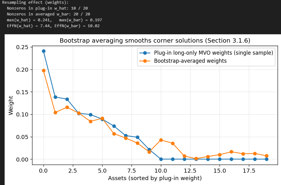
As you can see, half of the weights generated by the plug-in MVO are exactly zero, whereas with the bootstrap-averaged method, we have no zero weights. Those weights that are non-zero are also larger for the plug-in MVO. We are therefore better diversified using the bootstrap-averaged weights method.
Constraining and Regularizing the Optimizer
Even with improved inputs, the optimizer can still overreact. Constraining the optimization problem is therefore the second major lever. The guiding principle is simple: if you restrict the feasible set or penalize extreme solutions, the optimizer has fewer degrees of freedom to express estimation noise.
Box constraints, no-short constraints, and leverage limits
A basic set of implementability constraints is
along with the budget constraint 1^T w = 1. The no-short constraint is the special case (l_i = 0). A leverage constraint can be expressed as
When shorts are allowed, |w|_1 measures gross exposure; limiting it prevents the optimizer from creating offsetting long/short positions that are highly sensitive to small covariance or mean differences.
Why do these constraints work? They impose a cap on sensitivity. If the optimizer cannot push weights arbitrarily far, then errors in hat{mu} and hat{Sigma} cannot translate into arbitrarily extreme positions.
A common misconception is that constraints only reflect operational needs. In practice, they often serve a dual purpose: implementability and robustness.
Regularization Penalties: Making MVO behave like a well-posed estimation problem
Instead of hard constraints, one can add penalties to the objective. Consider augmenting (MVO-2) with an l2 (ridge) penalty:
Because |w|_2^2 = w^T I w, the risk term becomes
So ridge-regularized MVO is equivalent to replacing Sigma with
This is a profound and practical insight: a simple weight penalty is mathematically identical to eigenvalue inflation of the covariance matrix. It improves conditioning by pushing all eigenvalues away from zero, directly addressing the instability of Sigma^{-1}. In effect, it says: “do not trust low-variance directions too much; treat them as riskier than the raw estimate suggests.”
One can also use an l1 (lasso) penalty:
The l1 penalty encourages sparsity (many weights exactly zero) and discourages large gross exposure, especially when shorts are allowed. It is closely related to constraining |w|_1 as in (3.11). Sparse portfolios can be easier to implement and often exhibit lower turnover.
Note: if w >= 0 and 1^T w = 1, then |w|_1 = 1 is constant, so an l1 penalty on weights has no effect. l1 becomes meaningful when shorting is allowed (gross exposure varies), when applied to active weights a = w - w_b, or when penalizing turnover |w_t - w_{t-1}|_1.
Both l1 and l2 regularization can be understood as injecting a preference for “simple” portfolios, portfolios that do not require precise estimates to justify intricate long/short structures.
The following code demonstrates what happens if you adjust the ridge parameter lambda:
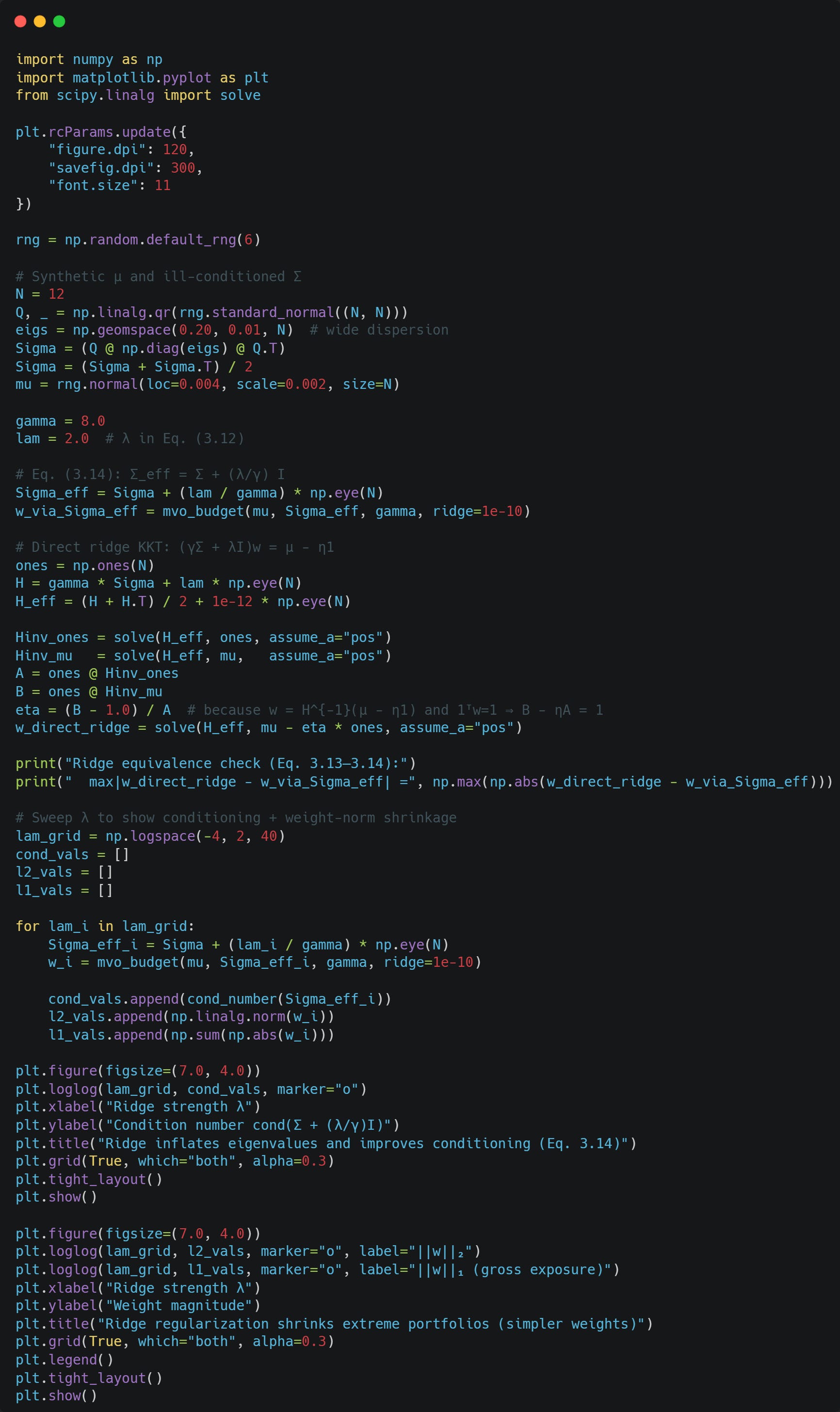
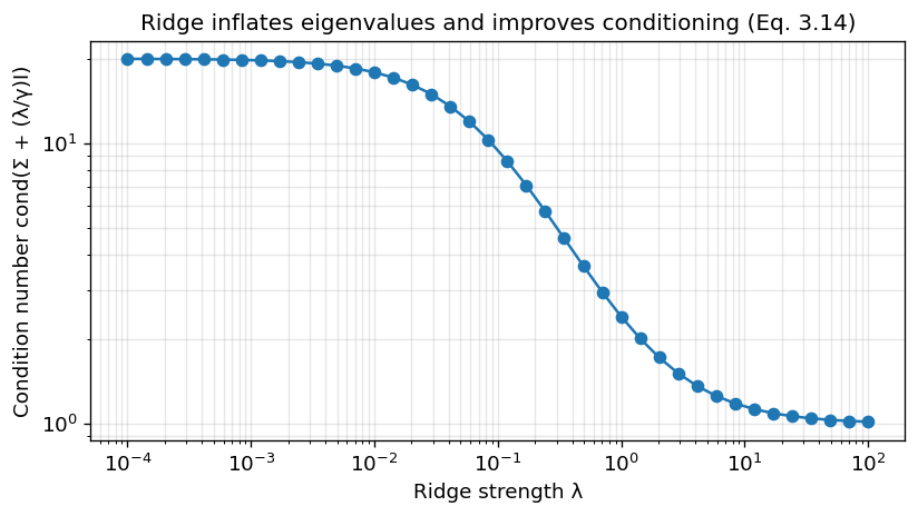
Higher lambda results in better conditioned Sigma.
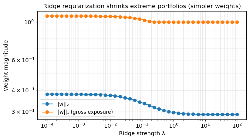
Higher lambda results in lower L1 and L2 norm of w (The portfolios become “simpler”).
Turnover and Transaction Costs: Regularizing changes the weights
A portfolio is rarely optimized once. In practice, we solve a sequence of problems over time. Estimation noise then manifests as unstable changes in weights, i.e., turnover.
A common fix is to add trading costs or turnover penalties. Let w_{t-1} be current holdings and w_t the new decision. A quadratic turnover penalty gives
This makes the optimizer “reluctant” to move unless the gain in mean–variance utility is large enough to justify the change. Importantly, this is also a robustness device: it prevents the optimizer from chasing small, noisy changes in hat{mu} or hat{Sigma}.
Linear cost models use |w_t - w_{t-1}|_1 instead, which can better capture proportional costs and induce sparse trading (only a subset of names trade each period).
The deeper point is that multi-period implementation turns MVO into a control problem. Regularizing the control (weight changes) is often more impactful than regularizing the state (weights) alone.
Let’s compare the evolution of two portfolios: One via regular MVO and one with the L1 penalty for weight changes. Let’s also see how changing kappa affects our portfolio.
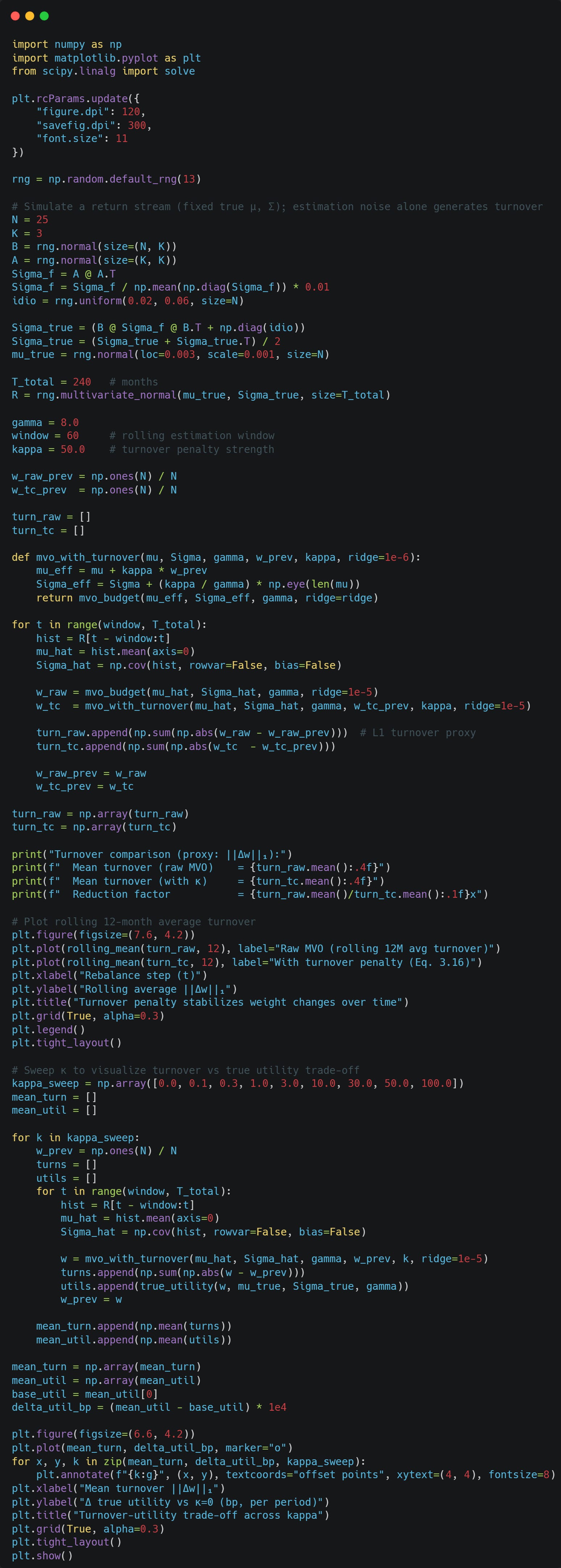
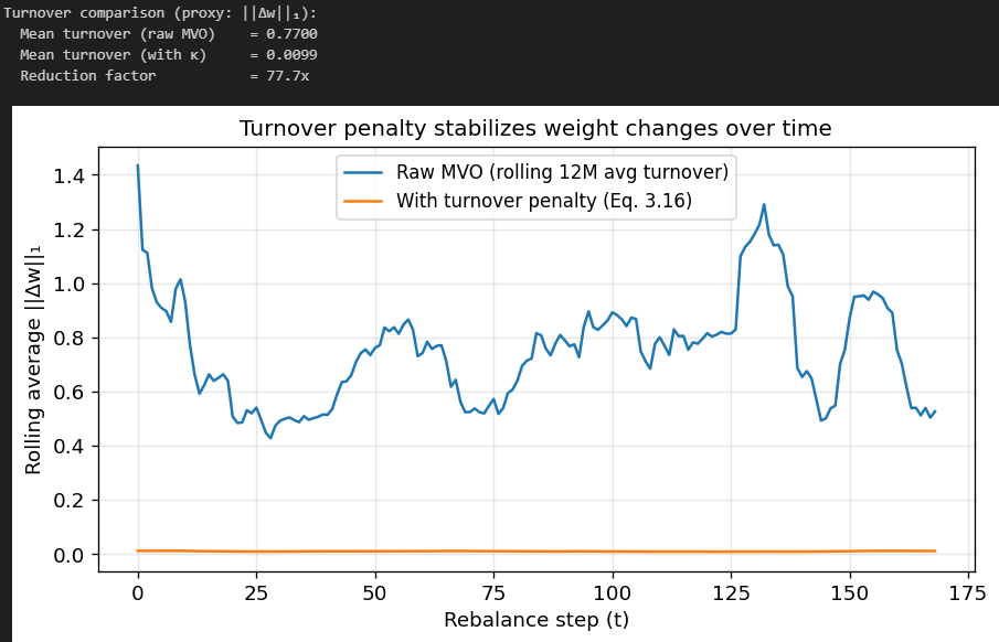
Above, we’ve used a kappa of 50. As you can see, turnover is very heavily reduced.
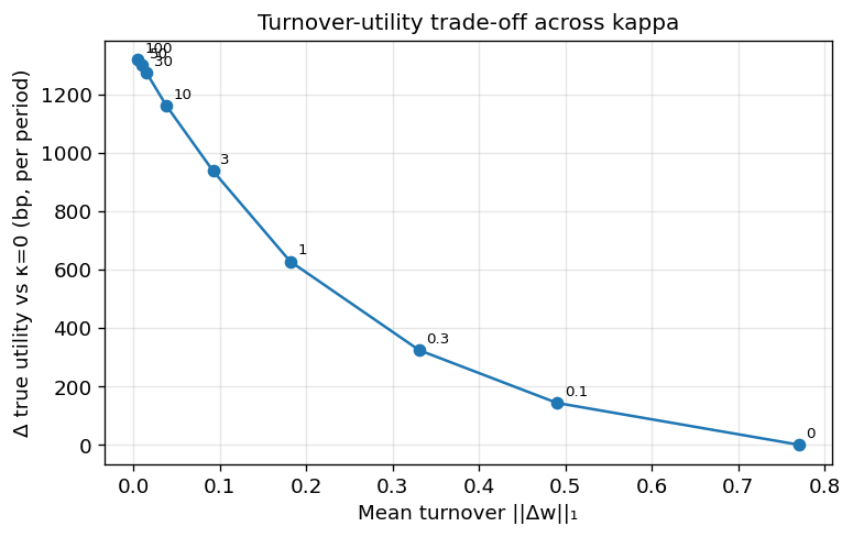
Here you can see that as you increase your turnover penalty kappa, your improvement vs an unpenalized portfolio becomes better and better, but returns are becoming diminishing with values >= 30.
In a real market that can change more abruptly, you may want to pick kappa slightly lower to be able to adapt more quickly.
Benchmark-relative optimization
Many institutional mandates are benchmark-relative. Let w_b be benchmark weights. Define active weights a = w - w_b. Then tracking error variance is
A common optimization is to maximize expected active return subject to tracking error:
where alpha represents expected alphas (expected excess returns relative to benchmark). This formulation has an important robustness advantage: it anchors the portfolio near a diversified benchmark, limiting the optimizer’s ability to create extreme positions driven by noise. In effect, the benchmark provides a strong prior on the weight vector.
Even if one is not formally benchmarked, this insight generalizes: anchoring optimization around a reference portfolio (market, equal weight, risk parity) often improves stability.
Robust Optimization: Optimizing against parameter uncertainty directly
A conceptually clean way to address estimation error is to incorporate uncertainty sets for mu and/or Sigma, then optimize a worst-case objective. This approach turns “garbage in, garbage out” into “uncertainty in, robustness out.”
One standard robust mean model assumes mu lies in an ellipsoid around hat{mu}:
Consider the robust counterpart of maximizing expected return minus risk, taking the worst-case mean:
The inner minimization has a closed form:
So the robust problem becomes
This is illuminating. The robust adjustment subtracts a term proportional to portfolio volatility, effectively reducing the attractiveness of portfolios whose expected return advantage might be explained by estimation error. The optimizer is forced to find portfolios whose expected return is high relative to uncertainty.
Robust covariance uncertainty sets lead to related regularization effects, often inflating risk in uncertain directions; again echoing the intuition behind shrinkage and ridge penalties. Robust optimization provides a principled bridge between statistical uncertainty and optimization regularization.
Let’s compare this to standard MVO:
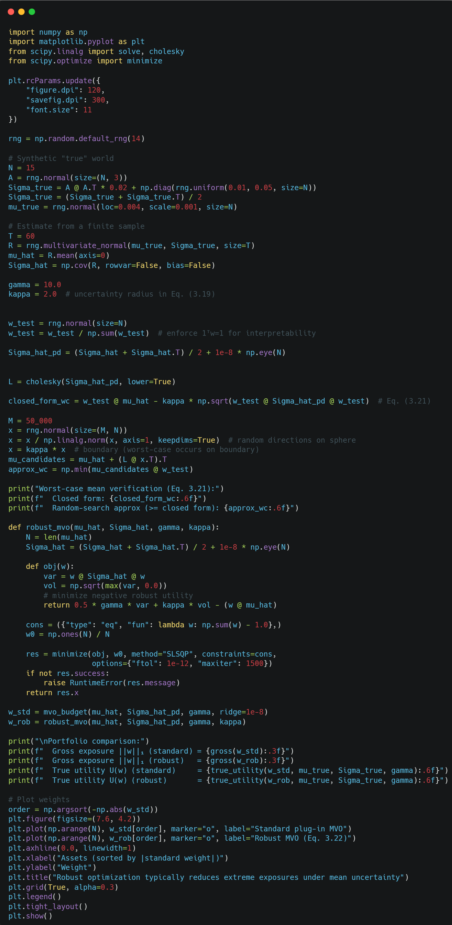
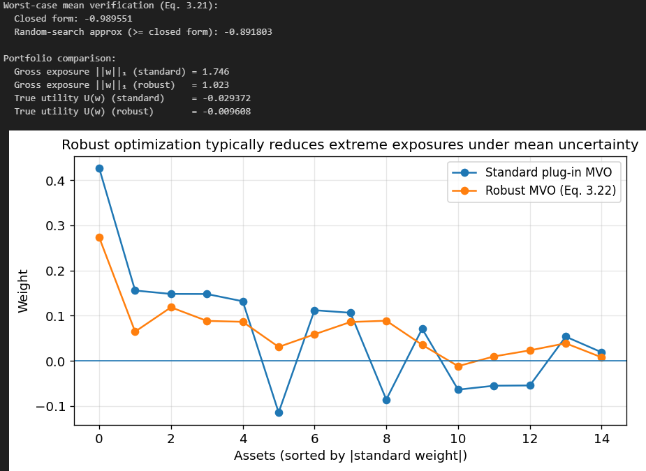
Our Robust MVO weights are a lot more “clean” compared to the standard MVO weights.
Conclusion
It is tempting to treat the practical modifications above as an ad hoc toolbox: shrinkage here, constraints there, turnover penalties elsewhere. A more coherent view is that these methods all solve the same underlying problem:
The plug-in MVO portfolio is a high-variance estimator of the optimal weights.
Reducing that variance requires injecting structure, equivalently, adding bias.
Shrinkage of Sigma reduces the variance of covariance estimates (and stabilizes inversion) at the cost of bias toward the target structure.
Factor models impose a low-rank structure that may be misspecified but dramatically reduces estimation noise.
Shrinkage and Bayesian methods for mu explicitly acknowledge that sample means are too noisy to trust fully.
Constraints and penalties reduce the effective degrees of freedom of the portfolio, preventing the optimizer from encoding noise into intricate weight patterns.
Turnover penalties reduce the variance of changes in weights, which is often the real operational pain point.
Robust optimization is an explicit uncertainty-aware form of regularization.
From this perspective, the “right” portfolio is not the one that is optimal for the estimated parameters; it is the one that is optimal for the decision problem under uncertainty, including estimation error, non-stationarity, and implementability constraints.
Quant Corner: https://discord.gg/X7TsxKNbXg
Code: https://gist.github.com/vertoxquant/e417b8afd2abe0e15ae0ff486813842a