
Backtests Lie: Building a Stress-Test Framework for Trading Signals
Synthetic nulls, falsification audits, and backtest inflation diagnostics in Python.

Look at this backtest I found online:
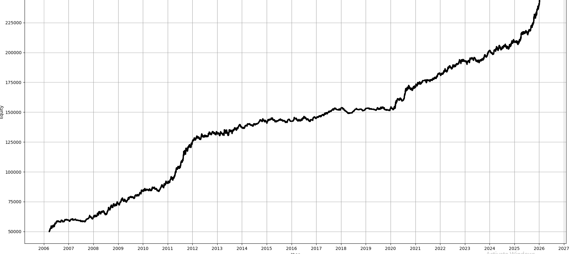
One of your first thoughts when looking at a stranger’s backtest is probably that it’s overfit, or that there is some look-ahead somewhere.
When you go a step further, you are probably constantly worried about overfitting your own backtests too!
In this article, we will introduce a framework that allows you to identify both! It’s a two-stage approach introduced in D. Nikolopoulos (2026). We will introduce the method, develop the two-stage approach, test the methodology empirically on a crypto dataset, look at some limitations, and also add some improvements of my own!
This article is free to read. You can support me immensely by sharing this article:
I write about quantitative trading the way it’s actually practiced:
Robust models and portfolios, combining signals and strategies, understanding the assumptions behind your models.
More broadly, I write about:
Statistical and cross-sectional arbitrage
Managing multiple strategies and signals
Risk and capital allocation
Research tooling and methodology
In-depth model assumptions and derivations
If this way of thinking resonates, you’ll probably like what I publish.
How Backtests Lie
There are three main failure modes in backtests: Leakage, selection bias, and specification error. Let’s go over them.
Leakage
Leakage is when you are making decisions based on information not yet available at that time. This doesn’t have to be something extreme like using future price data when calculating momentum, or using the current day’s low as a stop loss when still mid-day; it can be more subtle things like normalizing based on the full-sample volatility.
We can describe this mathematically with the help of filtrations. If you are unfamiliar with this concept, please read the following article:

A signal x_t is valid if and only if it is measurable with respect to F_{t-1}:
F_{t-1} reflects everything that is knowable at time t-1, like all past prices p_1, …, p_{t-1}, all past return r_1, …, r_{t-1}, all past volumes, etc.
As time progresses, it only grows:
You never forget information; you only accumulate more.
The full-sample normalization is NOT measurable:
since mu_T and sigma_t depend on observations you haven’t seen yet at time t. The correct expanding window version restores measurability:
Selection Bias
Selection bias, or overfitting, is when you test many different strategies (or configurations of one strategy) and report the best one. Even on a dataset that is not predictable at all, like white noise, this will produce performance better than 0.
Formally, assume returns follow a martingale difference sequence under the null hypothesis:
For each candidate strategy k, we compute its in-sample mean return R, and measure its statistical significance using a HAC t-statistic (A t-statistic that accounts for autocorrelation and heteroskedasticity commonly observed in financial markets):
where V_HAC is the Newey-West variance estimator. For more on Newest-West and HAC t-statistics, read the following article:

Under H_0, Z_{IS,k} is standard normally distributed asymptotically; values above 1.96 should only occur 5% of the time by chance.
But when you search over K configurations and always report the best one:
This grows with K even under H_0:
where gamma (the Euler-Mascheroni constant) is roughly 0.5772 and
This is a result of Extreme Value Theory; you don’t need to memorize the formula.
At K=100, your expected best t-statistic is already around 2.79, well above the 1.96 significance threshold.
Specification Error
Specification error is when your model technically makes money, but you misinterpret why it makes money.
A classic example of this is exposure to factors like market, momentum, liquidity, etc.
Formally, assume your returns follow the following factor model:
where f_t is a known risk factor, beta_t is your exposure to it, and alpha_t is the true time-varying alpha not captured by your factor (You can, of course, extend this to multiple factors). Specification error here would be thinking alpha_t is bigger than it actually is.
The second form of specification error is fitting a transient regime. Your model found a pattern specific to a particular market period or regime that doesn’t reflect a structural inefficiency. It worked in your backtest window, but it won’t persist in live trading.
Our Pipeline
Before going into the stress-test framework, let’s first introduce the pipeline we will test this on. We will explore a moving-average crossover strategy on daily BTCUSD data from CoinAPI, optimized and tested walk-forward with an In-sample of 2 years and an out-of-sample of 6 months.
df = pd.read_csv("C:\\QuantData\\CoinAPI Survivorship Bias Free\\BTC_USD_1DAY_COMPOSITE.csv").set_index("date")["close"]
returns = df.pct_change().dropna()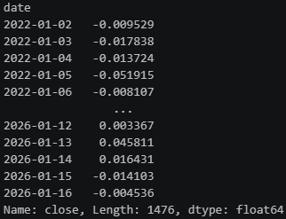
# --- Signal ---
def ma_signal(returns, short, long):
    prices = (1 + returns).cumprod()
    short_ma = prices.rolling(short).mean()
    long_ma = prices.rolling(long).mean()
    signal = np.where(short_ma > long_ma, 1, -1)
    return pd.Series(signal, index=returns.index)

# --- HAC t-statistic ---
def hac_tstat(rets, max_lag=None):
    T = len(rets)
    if max_lag is None:
        max_lag = int(4 * (T / 100) ** (2/9))
    mu = rets.mean()
    gamma0 = np.mean((rets - mu) ** 2)
    V_hac = gamma0
    for l in range(1, max_lag + 1):
        w = 1 - l / (max_lag + 1)
        gamma_l = np.mean((rets[l:] - mu) * (rets[:-l] - mu))
        V_hac += 2 * w * gamma_l
    return mu / np.sqrt(V_hac / T)

# --- Walk-Forward ---
def walk_forward(returns, in_sample_days=365*2, out_sample_days=180):
    short_grid = range(5, 51, 5)
    long_grid = range(20, 201, 20)

    results = []
    starts = range(0, len(returns) - in_sample_days - out_sample_days, out_sample_days)

    for start in starts:
        r_IS = returns.iloc[start : start + in_sample_days]
        r_OOS = returns.iloc[start + in_sample_days : start + in_sample_days + out_sample_days]

        best_z, best_short, best_long = -np.inf, None, None
        for s in short_grid:
            for l in long_grid:
                if s >= l:
                    continue
                sig = ma_signal(r_IS, s, l).shift(1).dropna()
                strat_rets = (r_IS * sig).dropna()
                if len(strat_rets) < 30:
                    continue
                z = hac_tstat(strat_rets)
                if z > best_z:
                    best_z = z
                    best_short, best_long = s, l

        sig_OOS = ma_signal(r_OOS, best_short, best_long).shift(1).dropna()
        strat_rets_OOS = (r_OOS * sig_OOS).dropna()
        z_OOS = hac_tstat(strat_rets_OOS)

        results.append({
            "start": returns.index[start],
            "best_short": best_short,
            "best_long": best_long,
            "z_IS": best_z,
            "z_OOS": z_OOS,
            "rets_OOS": strat_rets_OOS
        })

    return pd.DataFrame(results)
results = walk_forward(returns)
print(results[["start", "best_short", "best_long", "z_IS", "z_OOS"]])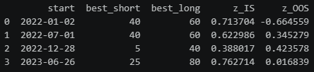
Stage 1: Falsification
The core idea of Stage 1 is simple: If your pipeline finds alpha in data where alpha cannot exist by construction, your pipeline is broken.
We introduce 5 null environments that try to target different failure modes:
Environment A: White Noise
Returns are i.i.d. Gaussian with zero mean:
Then
Annualized volatility target sigma_ann = 0.20, giving
If your pipeline finds alpha here, it is purely selection bias.
Let’s test our moving-average crossover walk-forward pipeline with this:
def generate_env_a(returns, sigma_ann=0.20, seed=None):
    if seed is not None:
        np.random.seed(seed)
    sigma_daily = sigma_ann / np.sqrt(365)
    null_returns = pd.Series(
        np.random.normal(0, sigma_daily, len(returns)),
        index=returns.index
    )
    return null_returns
null_rets = generate_env_a(returns, seed=42)
null_results = walk_forward(null_rets)
print(null_results[["start", "best_short", "best_long", "z_IS", "z_OOS"]])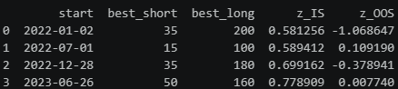
The results are exactly what we expect: In-sample Z_IS^* values between 0.58 and 0.77 reflect modest inflation from grid search, while out-of-sample Z_OOS values hover around zero. There is no consistent OOS edge.
Environment B: Regime-Switching Volatility
This environment detects predictability arising from improper normalization rules that leak future volatility states, regime leakage, or scale-based trading rules that inadvertently exploit volatility regimes. Let s_t in {1,2} be a two-state Markov chain with transition matrix
Returns are generated as
with epsilon_t independent of F_{t-1}^(r). Therefore E[r_t|F_{t-1}^(r)] = 0.
The paper chooses the following values:
Low-regime annualized volatility sigma_ann = 0.10, high regime volatility multiplier m=3.0, regime presistence p_11 = p_22 = 0.98. Hence
Here’s the implementation:
def generate_env_b(returns, p11=0.98, p22=0.98, sigma_ann_low=0.10, sigma_ann_high=0.30, seed=None):
    if seed is not None:
        np.random.seed(seed)
    sigma_low = sigma_ann_low / np.sqrt(365)
    sigma_high = sigma_ann_high / np.sqrt(365)

    T = len(returns)
    states = np.zeros(T, dtype=int)
    states[0] = 0
    for t in range(1, T):
        if states[t-1] == 0:
            states[t] = 0 if np.random.rand() < p11 else 1
        else:
            states[t] = 1 if np.random.rand() < p22 else 0

    sigmas = np.where(states == 0, sigma_low, sigma_high)
    null_returns = pd.Series(
        np.random.normal(0, sigmas),
        index=returns.index
    )
    return null_returns
null_rets_b = generate_env_b(returns, seed=42)
results_b = walk_forward(null_rets_b)
print(results_b[["start", "best_short", "best_long", "z_IS", "z_OOS"]])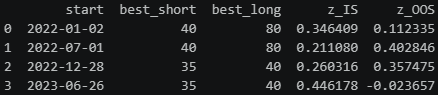
Environment C: Friction Placebo (Bid-Ask Bounce)
Let u_t be the latent efficient return, the “true” return of the asset satisfying the martingale null (E[u_t | F_{t-1}^(u)] = 0):
The observed return is then contaminated by bid-ask bounce via an MA(1) process:
The negative theta creates negative first-order autocorrelation in observed returns, which are predictable, but NOT tradable! Short-term mean reversion strategies suffer especially hard from this bias.
Innovations are scaled to match a target annualised volatility sigma_ann. Let
so that
The paper picks sigma_ann = 0.20 and theta = -0.5.
If your pipeline profits from this, it has timing errors, indexing bugs, or execution misalignment. Your pipeline isn’t statistically broken, but economically.
Note: We are working with daily prices here, where the bid-ask bounce is typically no longer significant.
Here’s the implementation:
def generate_env_c(returns, theta=-0.5, sigma_ann=0.20, seed=None):
    if seed is not None:
        np.random.seed(seed)
    sigma_daily = sigma_ann / np.sqrt(365)
    sigma_eps = sigma_daily / np.sqrt(1 + theta**2)

    T = len(returns)
    u = np.random.normal(0, sigma_eps, T + 1)
    r = u[1:] + theta * u[:-1]

    null_returns = pd.Series(r, index=returns.index)
    return null_returnsnull_rets_c = generate_env_c(returns, seed=42)
results_c = walk_forward(null_rets_c)
print(results_c[["start", "best_short", "best_long", "z_IS", "z_OOS"]])
null_rets_c = generate_env_c(returns, seed=42)
results_c = walk_forward(null_rets_c)
print(results_c[["start", "best_short", "best_long", "z_IS", "z_OOS"]])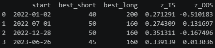
Environment D: Factor Null (One-Factor, Zero Alpha)
Returns are driven by a mean-zero risk factor with zero alpha:
with
and (f_t, e_t) independent of F_{t-1}^(r). Hence E[r_t |F_{t-1}^(r)] = 0.
The paper’s default calibration is beta = 1.0 and daily volatilities
This catches strategies mistaking beta for alpha. If your pipeline finds alpha here, it’s just harvesting systematic factor exposure rather than a genuine edge.
Here’s the implementation:
def generate_env_d(returns, beta=1.0, sigma_ann_f=0.20, sigma_ann_e=0.10, seed=None):
    if seed is not None:
        np.random.seed(seed)
    sigma_f = sigma_ann_f / np.sqrt(365)
    sigma_e = sigma_ann_e / np.sqrt(365)

    T = len(returns)
    f = np.random.normal(0, sigma_f, T)
    e = np.random.normal(0, sigma_e, T)
    r = beta * f + e

    null_returns = pd.Series(r, index=returns.index)
    return null_returns
null_rets_d = generate_env_d(returns, seed=42)
results_d = walk_forward(null_rets_d)
print(results_d[["start", "best_short", "best_long", "z_IS", "z_OOS"]])Environment E: Volatility Clustering Null (GARCH(1,1), Zero Mean)
This environment produces volatility clustering while preserving a zero conditional mean:
Conditional on F_{t-1}^(r), h_t is measurable and E[z_t] = 0, hence E[r_t | F_{t-1}^(r)] = 0.
The paper sets alpha = 0.10, beta = 0.85 (so alpha + beta = 0.95 < 1). They chose omega to match the target daily variance. Let
Then
When volatility is highly persistent (high alpha + beta), your return series has strong conditional heteroskedasticity. The HAC t-statistic assumes the variance estimator converges to the true long-run variance, but with finite OOS windows (6 months in our case) and persistent GARCH dynamics, the Newey-West estimator can underestimate the true variance, making your t-statistic look more significant than it really is. So we might report a significant Z_OOS^* not because we found alpha, but because the GARCH vol clustering causes the standard error to be underestimated, inflating the t-statistic artificially.
Here’s the implementation:
def generate_env_e(returns, alpha=0.10, beta=0.85, sigma_ann=0.20, seed=None):
    if seed is not None:
        np.random.seed(seed)
    sigma_daily = sigma_ann / np.sqrt(365)
    omega = (1 - alpha - beta) * sigma_daily**2

    T = len(returns)
    r = np.zeros(T)
    h = np.zeros(T)
    h[0] = sigma_daily**2

    z = np.random.normal(0, 1, T)
    for t in range(1, T):
        h[t] = omega + alpha * r[t-1]**2 + beta * h[t-1]
        r[t] = np.sqrt(h[t]) * z[t]

    null_returns = pd.Series(r, index=returns.index)
    return null_returns
null_rets_e = generate_env_e(returns, seed=42)
results_e = walk_forward(null_rets_e)
print(results_e[["start", "best_short", "best_long", "z_IS", "z_OOS"]])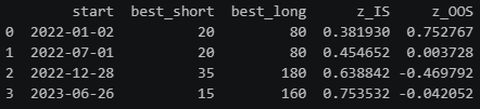
Full Stage 1 Run
So far, we’ve only tested one realization per null-environment, which can look good or bad by chance. It’s much better to run on each null environment M (= 100) times and compute Z_OOS^* for each run. The pipeline is falsified for the environment e if the fraction of runs exceeding 1.96 is significantly higher than 5%:
Under the null, this should be ~5% by construction. If it’s materially higher, your pipeline is systematically finding significance in null data, which means it’s broken.
Under the null, each run has a 5% chance of exceeding 1.96. With M=100 runs, the number of rejections follows
The 95th percentile of this distribution gives you the threshold that is exceeded only 5% of the time by chance.
Note: This part differs from how the paper things!
Let’s run this for our pipeline:
from scipy.stats import binom

def run_null_environment(generate_fn, returns, M=100, **kwargs):
    z_IS_list = []
    z_OOS_list = []

    for m in range(M):
        null_rets = generate_fn(returns, seed=m, **kwargs)
        results = walk_forward(null_rets)
        all_rets_OOS = pd.concat(results["rets_OOS"].tolist())
        z_star_IS = results["z_IS"].abs().mean()
        z_star_OOS = abs(hac_tstat(all_rets_OOS))
        z_IS_list.append(z_star_IS)
        z_OOS_list.append(z_star_OOS)

    return {
        "z_IS_mean": np.mean(z_IS_list),
        "z_IS_std": np.std(z_IS_list),
        "z_OOS_mean": np.mean(z_OOS_list),
        "z_OOS_std": np.std(z_OOS_list),
        "z_OOS_99pct": np.quantile(z_OOS_list, 0.99),
        "rejection_rate": np.mean(np.array(z_OOS_list) > 1.96)
    }

rejection_rate_threshold = binom.ppf(0.95, n=100, p=0.05) / 100

envs = {
    "A: White Noise": (generate_env_a, {}),
    "B: Regime Vol": (generate_env_b, {}),
    "C: Bid-Ask Bounce": (generate_env_c, {}),
    "D: Factor Null": (generate_env_d, {}),
    "E: GARCH": (generate_env_e, {})
}

rows = []
for name, (fn, kwargs) in envs.items():
    print(f"Running {name}...")
    res = run_null_environment(fn, returns, M=100, **kwargs)
    rows.append({"Environment": name, **res})

summary = pd.DataFrame(rows).set_index("Environment")
summary["Falsified"] = summary["rejection_rate"] > rejection_rate_threshold
print(f"\nRejection rate threshold (5% significance): {rejection_rate_threshold:.3f}")
print(summary[["z_IS_mean", "z_IS_std", "z_OOS_mean", "z_OOS_std", "z_OOS_99pct", "rejection_rate", "Falsified"]])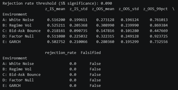
As you can see, our pipeline doesn’t have significantly high Z_OOS^* values. We can safely proceed to stage 2.
Stage 2: Inflation Quantification
Now that we know that our pipeline itself is not broken, we wanna figure out how inflated the in-sample results are.
Effective Multiplicity K_eff
When you search over K configurations and pick the best one, not all K configurations are truly independent. Two MA crossover strategies with parameters (10, 50) and (10, 60) will produce highly correlated return streams. Treating them as independent searches overstates how much you’ve actually explored the strategy space.
K_eff measures the true dimensionality of your search, how many genuinely independent configurations you actually tried.
Here’s how to compute it:
For each candidate configuration k, collect its in-sample return stream
Stack all K return streams into a T_{IS} x K matrix and compute the K x K correlation matrix Sigma, where entry (i,j) is the correlation between strategy i and strategy j’s returns.
The effective multiplicity is the spectral participation ratio of Sigma:
where lambda_i are the eigenvalues of Sigma. Since Sigma is a correlation matrix, we have tr Sigma = K, so
If all strategies are identical, one eigenvalue equals K, the rest are 0, so K_eff = 1.
If, on the other hand, all strategies are independent, all eigenvalues equal 1, and K_eff = K.
When K is large relative to your in-sample period T_IS, the sample correlation matrix becomes numerically unreliable. You can improve the reliability of your correlation matrix using shrinkage techniques, which I discuss in the following article:

Your expected best in-sample t-statistic under the null is
So K_eff directly determines how inflated your in-sample results are expected to be.
Now, different optimization techniques will yield different K_eff for the same K. A grid search is likely gonna result in a larger K_eff than Bayesian optimization with optuna. Let’s put this to the test. To prevent numerical issues, since we are working with daily data and only have 1477 observations, I will use the full dataset as an IS:
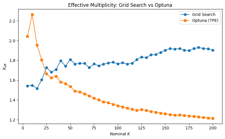
This result is REALLY interesting. Because optuna causes all our candidates to cluster in one space, K_eff actually DECREASES as you increase K. For grid search, it increases as expected. It’s also bigger than Grid Search for small values of K because it’s still in its exploration phase. TPE hasn’t accumulated enough trials to identify the promising region yet, so it samples more diversely across the parameter space. This gives a higher K_eff than grid search, which randomly but uniformly samples. As K grows, Optuna transitions to exploitation; it concentrates trials around the best configs it found, collapsing K_eff.
Our K_eff are also really small; we effectively only test 1-2 unique configurations. This makes sense with our simple moving average crossover strategy, though; there is not much variation across strategies.
Backtest Inflation: Delta Z
We now have a way to measure how many truly independent searches we performed. But we still need to quantify how much our in-sample result was inflated by that search.
The absolute magnitude gap Delta Z measures the divergence between your optimized in-sample evidence and its walk-forward realization:
Z_OOS^* stays bound regardless of how much you searched. Meanwhile, Z_IS^* grows with K_eff, so Delta Z directly captures the inflation induced by your search.
The expected Delta Z under the null, when there is no real alpha, is:
where sqrt(2/pi), around 0.80, is the expected absolute value of a standard normal, which Z_OOS^* should be under the null.
Let’s use this to test our walk-forward pipeline using both optuna and a grid-search for K=50:
def walk_forward_grid(returns, K=50, in_sample_days=365*2, out_sample_days=180):
    short_grid = range(2, 201, 1)
    long_grid = range(10, 1001, 1)
    configs = [(s, l) for s in short_grid for l in long_grid if s < l]
    np.random.seed(42)
    configs = [configs[i] for i in np.random.choice(len(configs), min(K, len(configs)), replace=False)]

    results = []
    starts = range(0, len(returns) - in_sample_days - out_sample_days, out_sample_days)

    for start in starts:
        r_IS = returns.iloc[start : start + in_sample_days]
        r_OOS = returns.iloc[start + in_sample_days : start + in_sample_days + out_sample_days]

        best_z, best_short, best_long = -np.inf, None, None
        for s, l in configs:
            sig = ma_signal(r_IS, s, l).shift(1).dropna()
            strat_rets = (r_IS * sig).dropna()
            if len(strat_rets) < 30:
                continue
            z = hac_tstat(strat_rets)
            if z > best_z:
                best_z = z
                best_short, best_long = s, l

        sig_OOS = ma_signal(r_OOS, best_short, best_long).shift(1).dropna()
        strat_rets_OOS = (r_OOS * sig_OOS).dropna()
        z_OOS = hac_tstat(strat_rets_OOS)

        results.append({
            "start": returns.index[start],
            "best_short": best_short,
            "best_long": best_long,
            "z_IS": best_z,
            "z_OOS": z_OOS,
            "rets_OOS": strat_rets_OOS
        })

    return pd.DataFrame(results)

def walk_forward_optuna(returns, K=50, in_sample_days=365*2, out_sample_days=180):
    results = []
    starts = range(0, len(returns) - in_sample_days - out_sample_days, out_sample_days)

    for start in starts:
        r_IS = returns.iloc[start : start + in_sample_days]
        r_OOS = returns.iloc[start + in_sample_days : start + in_sample_days + out_sample_days]

        def objective(trial):
            s = trial.suggest_int("short", 2, 200)
            l = trial.suggest_int("long", 10, 1000)
            if s >= l:
                return -np.inf
            sig = ma_signal(r_IS, s, l).shift(1)
            strat_ret = (r_IS * sig).dropna()
            if len(strat_ret) < 30:
                return -np.inf
            return hac_tstat(strat_ret)

        study = optuna.create_study(direction="maximize",
                                    sampler=optuna.samplers.TPESampler(seed=42))
        optuna.logging.set_verbosity(optuna.logging.WARNING)
        study.optimize(objective, n_trials=K)

        best_short = study.best_params["short"]
        best_long = study.best_params["long"]
        best_z = study.best_value

        sig_OOS = ma_signal(r_OOS, best_short, best_long).shift(1).dropna()
        strat_rets_OOS = (r_OOS * sig_OOS).dropna()
        z_OOS = hac_tstat(strat_rets_OOS)

        results.append({
            "start": returns.index[start],
            "best_short": best_short,
            "best_long": best_long,
            "z_IS": best_z,
            "z_OOS": z_OOS,
            "rets_OOS": strat_rets_OOS
        })

    return pd.DataFrame(results)

results_grid = walk_forward_grid(returns, K=50)
results_optuna = walk_forward_optuna(returns, K=50)

fig, axes = plt.subplots(1, 2, figsize=(12, 5))

for ax, (name, res) in zip(axes, [("Grid Search", results_grid), ("Optuna", results_optuna)]):
    delta_z = res["z_IS"] - res["z_OOS"]
    x = range(len(res))

    ax.bar(x, res["z_IS"], label="$Z^*_{IS}$", alpha=0.7)
    ax.bar(x, res["z_OOS"], label="$Z^*_{OOS}$", alpha=0.7)
    ax.axhline(0, color="black", linewidth=0.8)
    ax.set_xticks(list(x))
    ax.set_xticklabels(res["start"].tolist(), rotation=45, ha="right")
    ax.set_title(f"{name} — $\\Delta Z$ = {delta_z.mean():.2f}")
    ax.set_ylabel("$Z$")
    ax.legend()

plt.tight_layout()
plt.show()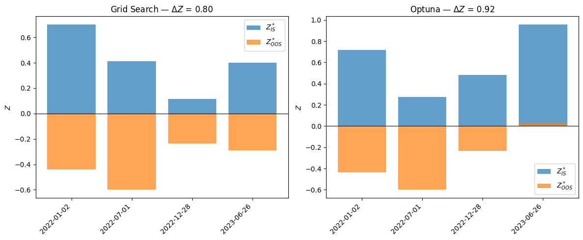
Both produce pretty bad strategies OOS. Let’s compare for different values of K now:
def theoretical_z_IS(keff):
    a = np.sqrt(2 * np.log(2 * keff)) - (np.log(np.log(2 * keff)) + np.log(4 * np.pi)) / (2 * np.sqrt(2 * np.log(2 * keff)))
    b = 1 / np.sqrt(2 * np.log(2 * keff))
    gamma = 0.5772
    return a + gamma * b

all_grid_results = {}
all_optuna_results = {}
all_keff_grid = {}
all_keff_optuna = {}

for K in K_values:
    print(f"K={K}...")
    all_grid_results[K] = walk_forward_grid(returns, K=K)
    all_optuna_results[K] = walk_forward_optuna(returns, K=K)
    all_keff_grid[K] = compute_keff(get_grid_search_returns(returns.iloc[:365*2], K))
    all_keff_optuna[K] = compute_keff(get_optuna_returns(returns.iloc[:365*2], K))

fig, axes = plt.subplots(4, 2, figsize=(12, 16))

for fold_idx in range(4):
    ax_z = axes[fold_idx, 0]
    ax_dz = axes[fold_idx, 1]

    grid_z_IS = [all_grid_results[K]["z_IS"].iloc[fold_idx] for K in K_values]
    optuna_z_IS = [all_optuna_results[K]["z_IS"].iloc[fold_idx] for K in K_values]
    theoretical_grid = [theoretical_z_IS(all_keff_grid[K]) for K in K_values]
    theoretical_optuna = [theoretical_z_IS(all_keff_optuna[K]) for K in K_values]
    grid_delta_z = [all_grid_results[K]["z_IS"].iloc[fold_idx] - all_grid_results[K]["z_OOS"].iloc[fold_idx] for K in K_values]
    optuna_delta_z = [all_optuna_results[K]["z_IS"].iloc[fold_idx] - all_optuna_results[K]["z_OOS"].iloc[fold_idx] for K in K_values]

    ax_z.plot(K_values, grid_z_IS, marker="o", label="Grid Search")
    ax_z.plot(K_values, optuna_z_IS, marker="s", label="Optuna (TPE)")
    ax_z.plot(K_values, theoretical_grid, linestyle="--", color="blue", label="Theoretical (Grid)")
    ax_z.plot(K_values, theoretical_optuna, linestyle="--", color="orange", label="Theoretical (Optuna)")
    ax_z.set_xlabel("Nominal $K$")
    ax_z.set_ylabel("$Z^*_{IS}$")
    ax_z.set_title(f"Fold {fold_idx + 1} — $Z^*_{{IS}}$")
    ax_z.legend()

    ax_dz.plot(K_values, grid_delta_z, marker="o", label="Grid Search")
    ax_dz.plot(K_values, optuna_delta_z, marker="s", label="Optuna (TPE)")
    ax_dz.set_xlabel("Nominal $K$")
    ax_dz.set_ylabel("$\\Delta Z$")
    ax_dz.set_title(f"Fold {fold_idx + 1} — $\\Delta Z$")
    ax_dz.legend()

plt.tight_layout()
plt.show()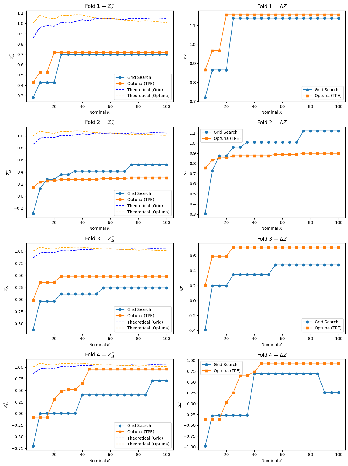
The theoretical scaling law is derived under the assumption that strategy returns are asymptotically Gaussian as T → infinity. In finite samples, especially with only 6 IS months, the HAC t-statistics have heavier tails than N(0,1), meaning the actual maximum Z_IS^* tends to be smaller than the Gaussian EVT formula predicts, making the theoretical bound conservative.
Your goal when designing a parameter optimization pipeline is to minimize Delta Z, while maximizing Z_OOS^*.
One decision rule for rejecting our pipeline could be:
Run M (= 100) white noise simulations, compute Delta Z for each, take the 99th percentile as your threshold, and if your observed Delta Z on real data exceeds this, falsify the pipeline.
Limitations
Sparse signals won’t be detected
If you have a strategy that rarely trades, like an event-based strategy, the walk-forward window simply won’t contain enough activations to reach significance even if the signal is genuine.
Passing doesn’t guarantee live performance
The audit is a stress test. A strategy can pass all 5 null environments, have a small Delta Z, and still lose money in live trading due to regime changes, liquidity constraints, or market impact. The audit only tells you your pipeline isn’t obviously broken.
Only for return prediction
The framework, as implemented, is designed for directional strategies with a well-defined trading lag. It doesn’t directly extend to portfolio optimization, classification tasks, volatility forecasting, or multi-asset strategies without adaptation.
Conclusion
Most quant researchers stress test their strategies manually and sporadically. This falsification framework can be permanently built into your research pipeline, running automatically every time you evaluate a new strategy or retune an existing one. Think of it like unit tests in software engineering: you don’t run them once before shipping, you run them on every commit.
Concretely, this means: every time your walk-forward backtest completes, Stage 1 and Stage 2 run automatically alongside it. Your research dashboard shows not just the equity curve and Sharpe ratio, but K_eff, Delta Z, and the Stage 1 rejection rates for all 5 environments. A strategy only advances to paper trading if it passes all steps, not because it looked good in-sample.
Join Quant Corner: https://discord.gg/X7TsxKNbXg
I’m first