
Fast Option Pricing using Fourier Transform
When Monte-Carlo is too slow

Monte-Carlo Simulation is the most straightforward way to price an option, and if you don’t care about speed, it’s a solid choice.
The moment you care about speed, like when quoting live, or when calibrating a pricing model where you need to reprice options thousands of times, Monte Carlo quickly becomes unusable.
This article presents three Fourier-based methods that solve this problem, reducing pricing from seconds to microseconds. We’ll use the Heston model as our running example throughout, and achieve a speedup of 30,000x against Monte Carlo!
I write about quantitative trading the way it’s actually practised:
Robust models and portfolios, combining signals and strategies, understanding the assumptions behind your models.
Topics I write about include portfolio construction, market making, risk management, research methodology, and more.
If this way of thinking resonates, you’ll probably like what I publish.
What you’ll learn
Why Monte Carlo breaks down for live pricing and model calibration, and what makes it fundamentally unsuitable for production options trading.
How the Fourier Transform and FFT work and why they matter for options pricing.
What the characteristic function is and how it enables us to price options even when the risk-neutral density of the model has no known closed-form analytical solution.
How Carr-Madan transforms option pricing into an FFT problem.
How Lewis reformulates the same problem via contour integration, eliminating the dampening parameter that makes Carr-Madan brittle.
How the COS method takes a completely different approach, approximating the density via a cosine series, and why it converges exponentially fast.
Python implementations for all methods, together with speed comparisons.
This article is free to read, so I would appreciate it if you shared it with someone who would also like it!
The Characteristic Function
To price options using Fourier methods, we need one thing from our model: the characteristic function of log S_T where S_T is the price at expiry.
For a random variable X, the characteristic function is defined as:
For log S_T we write:
where Q is the risk-neutral measure.
Just like the probability density function, it completely characterises the distribution of X. But while the density q(x) often has no closed-form expression, the characteristic function often does and is much easier to find.
In fact, the characteristic function and the density are a Fourier transform pair. Given the characteristic function, you can recover the density via the inverse Fourier transform:
This is the core idea behind all Fourier pricing methods. You don’t need to know the distribution of log S_T explicitly; you just need the characteristic function.
Why does the characteristic function always exist?
For any model where log S_T is a well-defined random variable, the characteristic function is guaranteed to exist for all real u, since
and thus the expectation is always finite.
Pricing in Fourier Space
In theory, you could now go ahead and compute the distribution from the characteristic function numerically, and then integrate against the payoff to get the fair value of the option. In practice, Fourier pricing methods skip this step entirely and price directly in Fourier space, which is both faster and more numerically stable.
Two Examples
For Black-Scholes, log S_T is Gaussian, so the characteristic function is that of a Gaussian random variable, with appropriate mean and standard deviation plugged in:
For Heston, log S_T has no nice closed-form density expression. But the characteristic function is still available in closed form:
where:
with
These are derived by applying Itô’s lemma to log S_t, exploiting the affine structure of the Heston dynamics, and solving the resulting Riccati ODEs in closed form.
How to properly derive this will be the subject of future articles.
Fourier Transform and FFT
Before deriving any pricing formulas, we need to understand the Fourier Transform and the Fast Fourier Transform algorithm.
The Fourier Transform
For a real square integrable function f(x), the Fourier transform is:
This function lives in frequency space; It tells you how much of each frequency xi is present in f. You recover f from hat{f} via the inverse Fourier transform:
Two real functions f and g that are both square integrable have a well-defined inner product. Parseval’s theorem says this inner product can also be computed in Fourier space:
This will be used later on in the Lewis method.
The Discrete Fourier Transform
In practice, you work with a finite grid of N points rather than a continuous function. The Discrete Fourier Transform (DFT) of a sequence x_0, x_1, …, x_{N-1} is:
Each output X_k is the inner product of the input sequence against a complex exponential at frequency k. Computing all N outputs naively requires evaluating N terms for each of the N outputs, a total of N^2 multiplications.
The Fast Fourier Transform
For N a power of 2, the Fast Fourier Transform, introduced by Cooley and Tukey, reduces the cost from O(N^2) to O(N log N) by exploiting the fact that the DFT of a sequence of length N can be written as the sum of two DFTs of length N/2.
Applying this decomposition recursively, splitting each half into its own two halves, reduces the total number of multiplications to O(N log N). For N = 4096, this is roughly a 340x speedup over the naive approach!
More formally, the DFT of a sequence of length N can be written as the sum of the DFT over the even-indexed elements and the DFT over the odd-indexed elements:
where E_k and O_k are the DFTs of the even and odd subsequences.
Carr-Madan
The Carr-Madan method (1999) is one of the most popular option pricing methods using the Fast Fourier Transform.
Let s = log S_T and k = log K. The risk-neutral density of s is q_T(s), with characteristic function
The call price as a function of log strike is:
We want to Fourier transform C_T(k). The problem is that C_T(k) is not square-integrable, since as k→ -infinity, C_T(k) → S_0 rather than decaying to zero. So its Fourier Transform doesn’t exist in the classical sense.
The fix is to multiply by an exponential dampening factor. Define the modified call price:
For suitable alpha, c_T(k) is square integrable, since the e^{alpha k) term decays fast enough as k → -infty to kill the blow-up. Therefore, this has a well-defined Fourier transform:
Our goal now is to write an analytical expression of Psi_T in terms of phi_T, and then obtain call prices numerically using the inverse transform.
Deriving Psi_T
Substitute the definitions of c_T(k) and C_T(k):
The region of integration is
which is equivalent to:
The integrand is non-negative, so we can apply Tonelli’s theorem and swap the order of integration:
Expand the inner integrand:
For the first term:
For the second term:
Substituting back:
Factor out
and recognise that since
we have:
So:
After simplifying, we finally get:
This is expressed entirely in terms of phi_T, the characteristic function of log S_T under our model of choice, which we said earlier we often have a closed-form solution for, so this whole thing is closed-form!
Recovery Formula
Since Psi_T is the Fourier transform of the dampened call price, standard Fourier inversion gives:
Dividing both sides by e^{alpha k}:
Since C_T(k) is real, we have
so the integrand over (-infty, 0) is the complex conjugate of the integrand over (0,infty), and their sum is twice the real part:
Choice of alpha
Two conditions constrain alpha. First, for Psi_T(0) to be finite, we need
Another condition is alpha not being equal to 0, to avoid a singularity in the denominator at v = 0. For Black-Scholes and Heston, all positive moments exist, so alpha is unconstrained. Carr and Madan suggest using one quarter of the upper bound implied by the moment condition, and find alpha = 1.5 works well in practice.
Truncation bound
The recovery integral runs from 0 to infinity. We need to verify it converges and can be safely truncated at some finite value a. For that, let’s first look at the numerator of |Psi_T(v)|.
It’s easy to see that
which is independent of v.
The denominator of Psi_T(v) grows like v^4 for large v, so:
for some constant A. Therefore
and the tail integral from any truncation point a satisfies:
Thus, the truncation error is bounded by:
To achieve a target error epsilon, choose:
FFT discretization
Discretize the recovery integral with N points at spacing eta, setting
Applying the trapezoid rule:
The effective upper limit of integration is a = N*eta. We want to evaluate this at a grid of N log-strikes
which gives us log strike levels ranging from -b to b, centred around ATM by setting
Substituting v_j and k_u:
For the sum to match the DFT structure
we need
This is the grid coupling constraint; Fine integration grid (eta small) forces coarse strike spacing (lambda large) and vice versa. The sum becomes:
which is exactly the DFT of the sequence
A single FFT call evaluates this for all N strikes simultaneously.
So you build the input vector
once and then call the FFT algorithm. Then multiply the u-th output by
to get the final call prices for each strike.
Simpson’s rule
The trapezoid rule has errors O(eta^2). To get accurate integration with larger eta, which, via the grid coupling constraint, means finer strike spacing, we replace the uniform weight eta with Simpson’s rule weights:
where delta_{j-1} is the Kronecker delta, equal to 1 only at j=1. The error improves from O(eta^2) to O(eta^4), and the FFT structure is preserved since replacing eta with w_j just multiplies each term by a scalar before applying the FFT.
The final formula is:
The weakness of Carr-Madan
The grid coupling constraint is the fundamental limitation; you cannot independently choose integration accuracy and strike grid density. Additionally, alpha requires model-specific tuning. Both issues are addressed by the methods that follow.
Python Implementation
We will be working with Heston in this article. Let’s first implement Monte Carlo pricing using Euler-Maruyama as a ground truth (note that Monte Carlo will give you slightly wrong values since we did not account for the discretisation, but it’s a method that is easy to implement and thus almost true, very likely) and for speed comparison:
import numpy as np
from scipy.stats import norm
import time
import matplotlib.pyplot as plt
from scipy.integrate import quad
def heston_mc(S0, K, r, q, T, kappa, theta, eta, rho, v0,
n_steps=200, n_paths=1_000_000, seed=42):
rng = np.random.default_rng(seed)
dt = T / n_steps
S = np.full(n_paths, float(S0))
v = np.full(n_paths, float(v0))
for _ in range(n_steps):
Z1 = rng.standard_normal(n_paths)
Z2 = rho * Z1 + np.sqrt(1 - rho**2) * rng.standard_normal(n_paths)
v_pos = np.maximum(v, 0)
S *= np.exp((r - q - 0.5 * v_pos) * dt + np.sqrt(v_pos * dt) * Z1)
v += kappa * (theta - v_pos) * dt + eta * np.sqrt(v_pos * dt) * Z2
return np.exp(-r * T) * np.mean(np.maximum(S - K, 0))Next, we implement the Heston Characteristic Function:
def heston_cf(omega, S0, r, q, T, kappa, theta, eta, rho, v0):
    x  = np.log(S0)
    xi = kappa - 1j * rho * eta * omega
    d  = np.sqrt(xi**2 + eta**2 * (omega**2 + 1j * omega))
    g  = (xi - d) / (xi + d)

    C = ((r - q) * 1j * omega * T
         + (kappa * theta / eta**2) * (
             (xi - d) * T - 2 * np.log((1 - g * np.exp(-d * T)) / (1 - g))
         ))
    D = ((xi - d) / eta**2) * (1 - np.exp(-d * T)) / (1 - g * np.exp(-d * T))

    return np.exp(C + D * v0 + 1j * omega * x)
and finally, the FFT implementation of Carr-Madan using Simpson weights:
def carr_madan_fft(S0, r, q, T, kappa, theta, eta, rho, v0,
                   alpha=1.5, N=4096, eta_grid=0.25):
    lam = 2 * np.pi / (N * eta_grid)
    b   = 0.5 * N * lam

    j   = np.arange(1, N + 1)
    v_j = eta_grid * (j - 1)

    cf  = lambda omega: heston_cf(omega, S0, r, q, T, kappa, theta, eta, rho, v0)

    psi = (np.exp(-r * T) * cf(v_j - (alpha + 1) * 1j)
           / (alpha**2 + alpha - v_j**2 + 1j * (2 * alpha + 1) * v_j))

    w   = (eta_grid / 3) * (3 + (-1)**j - (j == 1).astype(float))
    k_u = -b + lam * (np.arange(1, N + 1) - 1)

    x       = np.fft.fft(np.exp(1j * b * v_j) * psi * w)
    calls   = (np.exp(-alpha * k_u) / np.pi) * np.real(x)
    strikes = np.exp(k_u)

    return strikes, calls
Let’s compare MC to Carr-Mada:
# ── parameters ───────────────────────────────────────────────────────────────

params = dict(S0=100, r=0.05, q=0, T=1.0,
              kappa=2.0, theta=0.04, eta=0.3, rho=-0.7, v0=0.04)

strikes_to_price = np.arange(60, 141, 5, dtype=float)

# ── MC ground truth ───────────────────────────────────────────────────────────

t0 = time.perf_counter()
mc_prices = np.array([heston_mc(**params, K=K) for K in strikes_to_price])
mc_time   = time.perf_counter() - t0

# ── Carr-Madan ────────────────────────────────────────────────────────────────

t0 = time.perf_counter()
cm_strikes, cm_calls = carr_madan_fft(**params)
cm_time = time.perf_counter() - t0
cm_prices = np.interp(strikes_to_price, cm_strikes, cm_calls)

# ── print results ─────────────────────────────────────────────────────────────

print(f"{'Strike':>8} {'MC':>10} {'Carr-Madan':>12} {'Error':>10}")
print("-" * 44)
for K, mc, cm in zip(strikes_to_price, mc_prices, cm_prices):
    print(f"{K:>8.0f} {mc:>10.4f} {cm:>12.4f} {abs(mc-cm):>10.4f}")

print(f"\nMC time:          {mc_time:.2f}s  ({len(strikes_to_price)} strikes, 100k paths each)")
print(f"Carr-Madan time:  {cm_time*1000:.2f}ms (all strikes simultaneously)")

# ── plot ──────────────────────────────────────────────────────────────────────

fig, (ax1, ax2) = plt.subplots(1, 2, figsize=(12, 4))

ax1.plot(strikes_to_price, mc_prices, 'o', label='Monte Carlo', color='steelblue')
ax1.plot(strikes_to_price, cm_prices, '-', label='Carr-Madan', color='tomato', linewidth=2)
ax1.set_xlabel('Strike')
ax1.set_ylabel('Call Price')
ax1.set_title('Heston Call Prices')
ax1.legend()
ax1.grid(True, alpha=0.3)

ax2.bar(['Monte Carlo\n(100k paths, 17 strikes)', 'Carr-Madan FFT\n(all strikes)'],
        [mc_time, cm_time],
        color=['steelblue', 'tomato'])
ax2.set_ylabel('Time (seconds)')
ax2.set_title('Computation Time')
ax2.grid(True, alpha=0.3, axis='y')

plt.tight_layout()
plt.show()
Strike MC Carr-Madan Error
--------------------------------------------
60 43.0926 43.0487 0.0439
65 38.4447 38.4019 0.0428
70 33.8703 33.8281 0.0423
75 29.4033 29.3614 0.0420
80 25.0861 25.0447 0.0415
85 20.9701 20.9298 0.0403
90 17.1172 17.0758 0.0415
95 13.5838 13.5438 0.0401
100 10.4286 10.3950 0.0336
105 7.7081 7.6798 0.0283
110 5.4500 5.4306 0.0194
115 3.6676 3.6572 0.0104
120 2.3451 2.3334 0.0117
125 1.4146 1.4061 0.0085
130 0.8051 0.8002 0.0049
135 0.4343 0.4309 0.0034
140 0.2238 0.2206 0.0031
MC time: 6.46s (17 strikes, 100k paths each)
Carr-Madan time: 1.05ms (all strikes simultaneously)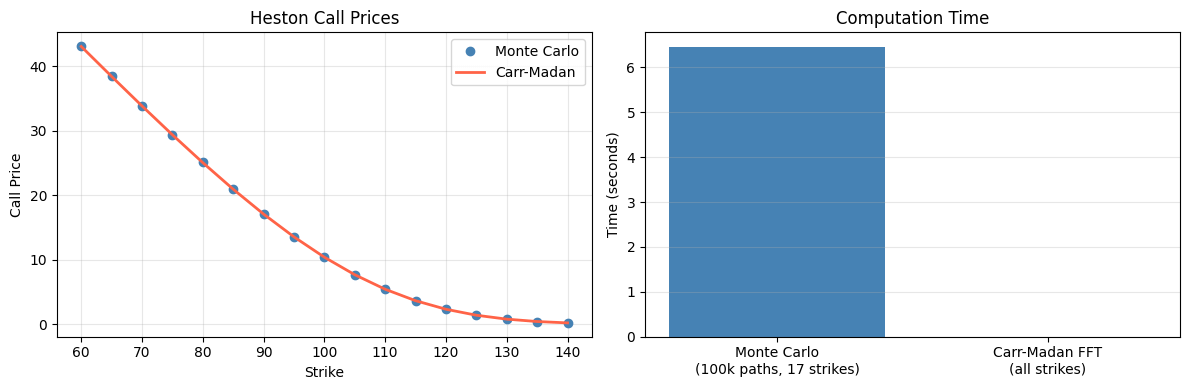
The results speak for themselves! Even at 100k paths, which isn’t all that much, and gives somewhat inaccurate results, running MC takes around 6.5 seconds, while Carr-Madan only takes a millisecond. But we can do even better!
Lewis
Lewis (2001) reformulates option pricing as a complex contour integral. The result is a cleaner formula than Carr-Mada; no dampening parameter alpha to tune, and the strip condition is easily satisfied for essentially all models used in practice.
The core idea
The option price is a discounted expectation under Q (We are restating this since the paper has slightly different notation):
where x = log S_T, w(x) is the payoff function, and q_T(x) is the risk-neutral density of log S_T. This is an inner product of w and q_T. Parseval’s theorem says inner products are preserved under Fourier transformation:
Since q_T(x) is real, we have
So:
The problem
That formula looks clean, but there’s a catch. For a call, the payoff is
which grows like e^x as x → infty. Its ordinary Fourier transform diverges!
Carr-Madan’s fix was to multiply the payoff by a dampening factor before transforming. Lewis takes a cleaner route: allow the transform variable to be complex.
Generalized Fourier Transform
Let z = u+iv be a complex number. Define the generalized Fourier transform of the payoff:
Now e^{izx} = e^{iux-vx}, and the factor e^{-vx} provides the decay that kills the growth of w(x), as long as v is large enough. For the call:
This does not converge unless Im(z) > 1. With Im(z) > 1 we have:
We call this area the strip of regularity for the call payoff:
You can refer to the following table from the paper for other options:
The characteristic function has its own regularity strip. For the characteristic function of X_T to exist, we need
The set of valid complex v with this property forms the strip S_X.
Define the reflected strip
This is where phi_T(-z) is regular, which is what appears in the pricing formula.
Shifting the contour
By Cauchy’s theorem, the integration contour may be shifted to any horizontal line inside the common strip of regularity:
The Lewis Formula
The option price finally becomes:
where v = Im(z) in S_V and Y = ln S_0 + (r-q)T is the log forward price, and phi denotes the characteristic function of the centred log-return X_T = log S_T - Y.
Call Pricing Formula
Substituting the call payoff transform hat{w} from above:
where b is some model-dependent upper bound below which the characteristic function stays regular. Lewi’s preferred contour is v=1/2, obtained by shifting the contour from (1,b) down to (0,1) via the residue theorem and picking up the pole at z=i. That gives
where k = ln(S_0/K) + (r-q)T is the log-moneyness. The contour v=1/2 sits symmetrically between the poles at z=0 and z=i, and requires only
satisfies by practically every standard model, and is a much weaker requirement than
that Carr-Madan needs for alpha > 0.
Python Implementation
Lewis uses the characteristic function of X_T:
def heston_cf_xt(omega, S0, r, q, T, kappa, theta, eta, rho, v0):
    """CF of X_T = log(S_T/S_0) - (r-q)T under Heston."""
    xi = kappa - 1j * rho * eta * omega
    d  = np.sqrt(xi**2 + eta**2 * (omega**2 + 1j * omega))
    g  = (xi - d) / (xi + d)

    C = (kappa * theta / eta**2) * (
            (xi - d) * T - 2 * np.log((1 - g * np.exp(-d * T)) / (1 - g))
        )
    D = ((xi - d) / eta**2) * (1 - np.exp(-d * T)) / (1 - g * np.exp(-d * T))

    # no (r-q) drift term since X_T is already centered
    return np.exp(C + D * v0 - 0.5 * 1j * omega * eta**2 * 0)
Now since Lewis doesn’t use FFT by design, we have to compute strikes one by one using the contour integral, or we are smart and vectorize:
def lewis_calls_vectorized(S0, strikes, r, q, T, kappa, theta, eta, rho, v0,
                           N=4096, eta_grid=0.25):
    u_j = eta_grid * np.arange(0, N)

    # Simpson weights
    w = np.ones(N) * 2
    w[1::2] = 4
    w[0] = w[-1] = 1
    w *= eta_grid / 3

    phi = heston_cf_xt(u_j - 0.5j, S0, r, q, T, kappa, theta, eta, rho, v0)
    phi /= (u_j**2 + 0.25)

    # k for each strike: shape (n_strikes,)
    k = np.log(S0 / strikes) + (r - q) * T

    # outer product: shape (n_strikes, N)
    phase = np.exp(1j * np.outer(k, u_j))

    I = np.real(phase * phi[np.newaxis, :]) @ w / np.pi

    return S0 * np.exp(-q * T) - np.sqrt(S0 * strikes) * np.exp(-(r + q) * T / 2) * I
And the comparison:
t0 = time.perf_counter()
lw_prices = lewis_calls_vectorized(strikes=strikes_to_price, **params)
lw_time = time.perf_counter() - t0

print(f"{'Strike':>8} {'MC':>10} {'Carr-Madan':>12} {'Lewis':>10} "
      f"{'CM Err':>10} {'LW Err':>10}")
print("-" * 64)
for K, mc, cm, lw in zip(strikes_to_price, mc_prices, cm_prices, lw_prices):
    print(f"{K:>8.0f} {mc:>10.4f} {cm:>12.4f} {lw:>10.4f} "
          f"{abs(mc-cm):>10.4f} {abs(mc-lw):>10.4f}")

print(f"\nMC time:          {mc_time:.2f}s")
print(f"Carr-Madan time:  {cm_time*1000:.2f}ms")
print(f"Lewis time:       {lw_time*1000:.2f}ms")

fig, (ax1, ax2) = plt.subplots(1, 2, figsize=(12, 4))

ax1.plot(strikes_to_price, mc_prices, 'o', label='Monte Carlo', color='steelblue')
ax1.plot(strikes_to_price, cm_prices, '-', label='Carr-Madan', color='tomato', linewidth=2)
ax1.plot(strikes_to_price, lw_prices, '--', label='Lewis', color='seagreen', linewidth=2)
ax1.set_xlabel('Strike')
ax1.set_ylabel('Call Price')
ax1.set_title('Heston Call Prices')
ax1.legend()
ax1.grid(True, alpha=0.3)

ax2.bar(['Carr-Madan\nFFT', 'Lewis\nVectorized'],
        [cm_time, lw_time],
        color=['tomato', 'seagreen'])
ax2.set_ylabel('Time (seconds)')
ax2.set_title('Computation Time (excl. Monte Carlo)')
ax2.grid(True, alpha=0.3, axis='y')

plt.tight_layout()
plt.show()
Strike MC Carr-Madan Lewis CM Err LW Err
----------------------------------------------------------------
60 43.0926 43.0487 43.1459 0.0439 0.0533
65 38.4447 38.4019 38.5020 0.0428 0.0573
70 33.8703 33.8281 33.9311 0.0423 0.0608
75 29.4033 29.3614 29.4673 0.0420 0.0640
80 25.0861 25.0447 25.1536 0.0415 0.0674
85 20.9701 20.9298 21.0417 0.0403 0.0716
90 17.1172 17.0758 17.1902 0.0415 0.0730
95 13.5838 13.5438 13.6612 0.0401 0.0774
100 10.4286 10.3950 10.5150 0.0336 0.0864
105 7.7081 7.6798 7.8025 0.0283 0.0944
110 5.4500 5.4306 5.5570 0.0194 0.1070
115 3.6676 3.6572 3.7858 0.0104 0.1182
120 2.3451 2.3334 2.4652 0.0117 0.1201
125 1.4146 1.4061 1.5412 0.0085 0.1266
130 0.8051 0.8002 0.9381 0.0049 0.1329
135 0.4343 0.4309 0.5717 0.0034 0.1375
140 0.2238 0.2206 0.3646 0.0031 0.1409
MC time: 8.09s
Carr-Madan time: 1.18ms
Lewis time: 2.49ms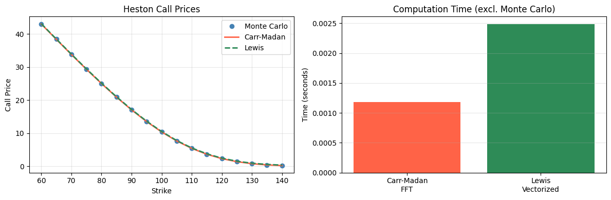
As you can see, when using the same N and eta as with Carr-Madan, Lewis starts diverging pretty quickly and is still over twice as slow. If we increase N and reduce eta, we are quickly multiple times slower than Carr-Madan when pricing many strikes at once. On the other hand, we get rid of the dampening parameter alpha, which can cause real problems.
Let’s finally look at our method of choice, which performs better than both Lewis and Carr-Madan.
The COS Method
Both Carr-Madan and Lewis price options by evaluating a Fourier integral numerically. The integrand is oscillatory, which is expensive to integrate accurately with equally spaced quadrature.
The COS method (2008) takes a different route. Instead of integrating the characteristic function directly, it expands the risk-neutral density in a cosine series and reads the series coefficients directly off the characteristic function, with those coefficients often being available analytically.
Fourier-Cosine Series Expansion
Starting from risk-neutral pricing (once again, slightly different notation!):
where x=ln(S_0/K), y = ln(S_T/K), v(y,T) is the payoff, and f(y|x) is the risk-neutral transition density of the log-return.
We truncate to a finite interval [a,b]:
Now expand f(y|x) in a cosine series on [a,b]:
where the ‘ in the sum means the k=0 term is weighted by 1/2, and the cosine coefficients are:
Substituting into the pricing integral and swapping sum and integral (which we can do thanks to Fubini):
where:
Note that the V_k are the cosine series coefficients of v(y,T) in y. Thus we have transformed the product of two real functions, f(y|x) and v(y,T), to that of their Fourier-cosine series coefficients.
Coefficients from the characteristic function
The density f(y|x) is unknown, that’s the whole reason we use Fourier methods in the first place. Comparing the definition of A_k(x) with the characteristic function phi_T(w), one finds that:
where phi_1 is the characteristic function computed over the truncated range [a,b]. Since [a,b] was chosen to capture essentially all the density mass, phi_1 is approx phi and so:
The COS Formula
Finally, replacing A_k by F_k in the formula for V(x, t_0), we obtain:
This is the COS formula.
Payoff coefficients for calls and puts
For a call, v(y,T) = K(e^y-1)^+, the integration domain reduces to [0,b] since the payoff is zero for y < 0. The coefficients are:
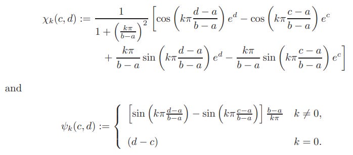
where chi and psi have closed forms:
For a put the integration domain is [a,0], and
In practice, you can price puts or calls, and recover the other via put-call parity
Truncation Range
The interval [a,b] must contain enough of the density without being so wide that the cosine approximation needs excessive terms to resolve the tails. Fang & Oosterlee propose using cumulants of ln(S_T/K):
where c_1, c_2, c_4 are the first, second and fourth cumulants of ln(S_T/K). Including c_4 matters for short maturities and fat-tailed processes where the density is sharply peaked.
You can additionally also include a c_6 term as well for extremely short maturities, but the sixth cumulant can be difficult to derive for many models. You can also go the other direction and only include the c_1 and c_2 terms.
Benefits of the COS method
For Carr-Madan and Lewis, accuracy is limited by how well a trapezoidal or Simpson sum approximates a slowly decaying oscillatory integral. The COS method avoids this entirely. For smooth densities like GBM, Heston, and many Lévy processes at moderate maturities, the density is C^{infty} on [a,b] and the cosine coefficients decay exponentially, yielding exponential convergence.
The computational complexity is O(N) for a single strike. For a vector of strikes, the F_k are the same across all strikes, and the V_k differ only through the x-dependent phase; pricing M strikes simultaneously costs O(MN) via matrix-vector multiplication.
Python Implementation
We need the first and second cumulants of log(S_T/K) under Heston:
def heston_cumulants(r, q, T, kappa, theta, eta, rho, v0):
    """First and second cumulants of log(S_T/K) under Heston."""
    c1 = (r - q) * T + (1 - np.exp(-kappa * T)) * (theta - v0) / (2 * kappa) - 0.5 * theta * T

    c2 = (1 / (8 * kappa**3)) * (
        eta * T * kappa * np.exp(-kappa * T) * (v0 - theta) * (8 * kappa * rho - 4 * eta)
        + kappa * rho * eta * (1 - np.exp(-kappa * T)) * (16 * theta - 8 * v0)
        + 2 * theta * kappa * T * (-4 * kappa * rho * eta + eta**2 + 4 * kappa**2)
        + eta**2 * ((theta - 2 * v0) * np.exp(-2 * kappa * T)
                    + theta * (6 * np.exp(-kappa * T) - 7) + 2 * v0)
        + 8 * kappa**2 * (v0 - theta) * (1 - np.exp(-kappa * T))
    )

    return c1, c2
Fast vectorized implementation of the COS method:
def cos_calls(S0, strikes, r, q, T, kappa, theta, eta, rho, v0, N=128, L=12):
    c1, c2 = heston_cumulants(r, q, T, kappa, theta, eta, rho, v0)
    a = c1 - L * np.sqrt(abs(c2))
    b = c1 + L * np.sqrt(abs(c2))

    k     = np.arange(N)
    omega = k * np.pi / (b - a)

    def varphi(omega):
        xi = kappa - 1j * rho * eta * omega
        d  = np.sqrt(xi**2 + eta**2 * (omega**2 + 1j * omega))
        g  = (xi - d) / (xi + d)
        C  = ((r - q) * 1j * omega * T
              + (kappa * theta / eta**2) * (
                  (xi - d) * T - 2 * np.log((1 - g * np.exp(-d * T)) / (1 - g))
              ))
        D  = ((xi - d) / eta**2) * (1 - np.exp(-d * T)) / (1 - g * np.exp(-d * T))
        return np.exp(C + D * v0)

    def chi(c, d):
        kpi = np.where(k != 0, omega, 1.0)
        val = (np.cos(kpi * (d - a)) * np.exp(d)
             - np.cos(kpi * (c - a)) * np.exp(c)
             + kpi * np.sin(kpi * (d - a)) * np.exp(d)
             - kpi * np.sin(kpi * (c - a)) * np.exp(c)) / (1 + kpi**2)
        val[0] = np.exp(d) - np.exp(c)
        return val

    def psi(c, d):
        val      = np.empty(N)
        val[0]   = d - c
        val[1:]  = (b - a) / (k[1:] * np.pi) * (
                       np.sin(omega[1:] * (d - a)) - np.sin(omega[1:] * (c - a))
                   )
        return val

    # precompute strike-independent quantities
    basis    = varphi(omega) * np.exp(-1j * omega * a)  # vphi * e^{-i*omega*a}
    A        = np.real(basis)
    B        = np.imag(basis)
    Uk       = (2 / (b - a)) * (-chi(a, 0) + psi(a, 0))

    # cache constants
    disc     = np.exp(-r * T)
    fwd_S0   = S0 * np.exp(-q * T)
    disc_K   = np.exp(-r * T)

    # vectorize over strikes
    x        = np.log(S0 / strikes)                    # shape (M,)
    theta_mx = np.outer(x, omega)                      # shape (M, N)
    F        = A * np.cos(theta_mx) - B * np.sin(theta_mx)  # shape (M, N)
    F[:, 0] *= 0.5

    puts  = disc * strikes * (F @ Uk)
    calls = puts + fwd_S0 - strikes * disc_K
    return calls
And last but not least, the comparison code:
t0 = time.perf_counter()
cos_prices = cos_calls(strikes=strikes_to_price, **params)
cos_time = time.perf_counter() - t0

print(f"{'Strike':>8} {'MC':>10} {'Carr-Madan':>12} {'Lewis':>10} {'COS':>10} "
      f"{'CM Err':>10} {'LW Err':>10} {'COS Err':>10}")
print("-" * 84)
for K, mc, cm, lw, cos in zip(strikes_to_price, mc_prices, cm_prices, lw_prices, cos_prices):
    print(f"{K:>8.0f} {mc:>10.4f} {cm:>12.4f} {lw:>10.4f} {cos:>10.4f} "
          f"{abs(mc-cm):>10.4f} {abs(mc-lw):>10.4f} {abs(mc-cos):>10.4f}")

print(f"\nMC time:          {mc_time:.2f}s")
print(f"Carr-Madan time:  {cm_time*1000:.2f}ms")
print(f"Lewis time:       {lw_time*1000:.2f}ms")
print(f"COS time:         {cos_time*1000:.2f}ms")

fig, (ax1, ax2) = plt.subplots(1, 2, figsize=(12, 4))

ax1.plot(strikes_to_price, mc_prices, 'o', label='Monte Carlo', color='steelblue')
ax1.plot(strikes_to_price, cm_prices, '-', label='Carr-Madan', color='tomato', linewidth=2)
ax1.plot(strikes_to_price, lw_prices, '--', label='Lewis', color='seagreen', linewidth=2)
ax1.plot(strikes_to_price, cos_prices, ':', label='COS', color='purple', linewidth=2)
ax1.set_xlabel('Strike')
ax1.set_ylabel('Call Price')
ax1.set_title('Heston Call Prices')
ax1.legend()
ax1.grid(True, alpha=0.3)

ax2.bar(['Carr-Madan\nFFT', 'Lewis\nVectorized', 'COS'],
        [cm_time, lw_time, cos_time],
        color=['tomato', 'seagreen', 'purple'])
ax2.set_ylabel('Time (seconds)')
ax2.set_title('Computation Time (excl. Monte Carlo)')
ax2.grid(True, alpha=0.3, axis='y')

plt.tight_layout()
plt.show()
Strike MC Carr-Madan Lewis COS CM Err LW Err COS Err
------------------------------------------------------------------------------------
60 43.0926 43.0487 43.1459 43.0487 0.0439 0.0533 0.0439
65 38.4447 38.4019 38.5020 38.4019 0.0428 0.0573 0.0428
70 33.8703 33.8281 33.9311 33.8280 0.0423 0.0608 0.0424
75 29.4033 29.3614 29.4673 29.3612 0.0420 0.0640 0.0421
80 25.0861 25.0447 25.1536 25.0446 0.0415 0.0674 0.0416
85 20.9701 20.9298 21.0417 20.9297 0.0403 0.0716 0.0403
90 17.1172 17.0758 17.1902 17.0753 0.0415 0.0730 0.0419
95 13.5838 13.5438 13.6612 13.5434 0.0401 0.0774 0.0404
100 10.4286 10.3950 10.5150 10.3942 0.0336 0.0864 0.0344
105 7.7081 7.6798 7.8025 7.6788 0.0283 0.0944 0.0293
110 5.4500 5.4306 5.5570 5.4303 0.0194 0.1070 0.0197
115 3.6676 3.6572 3.7858 3.6562 0.0104 0.1182 0.0114
120 2.3451 2.3334 2.4652 2.3326 0.0117 0.1201 0.0125
125 1.4146 1.4061 1.5412 1.4057 0.0085 0.1266 0.0089
130 0.8051 0.8002 0.9381 0.7996 0.0049 0.1329 0.0055
135 0.4343 0.4309 0.5717 0.4303 0.0034 0.1375 0.0039
140 0.2238 0.2206 0.3646 0.2203 0.0031 0.1409 0.0035
MC time: 8.09s
Carr-Madan time: 1.18ms
Lewis time: 2.49ms
COS time: 0.34ms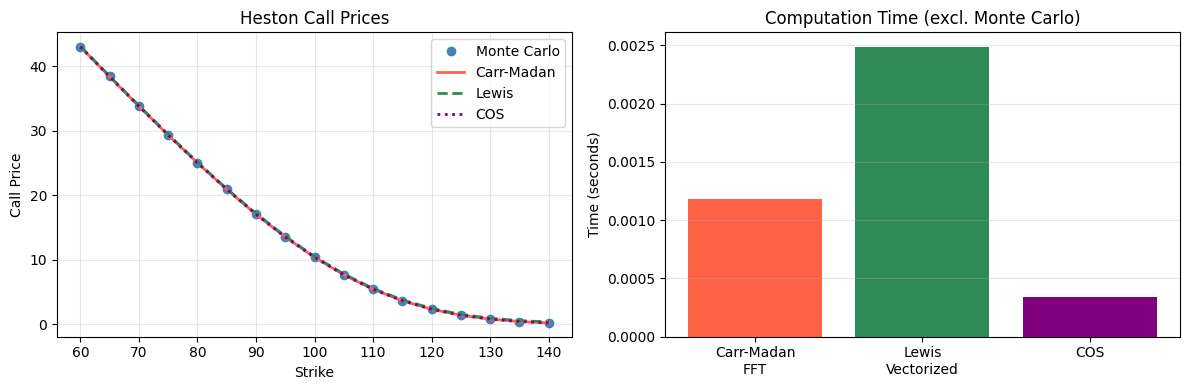
Awesome! We are more than 3 times faster than Carr-Madan, while getting rid of annoying parameters and gaining exponential convergence!
The method naturally vectorizes into dense linear algebra operations, meaning you could still make this way way faster if you optimized it properly.
Conclusion
Apologies for the delay since the last article! This one took a little longer than I expected since I had to verify all the math, and turn 3 papers into one article instead of the usual one paper.
I hope you enjoyed this rather math-heavy article anyway! I plan on covering more options content soon.
Other Articles You Would Enjoy


Quant Corner
Join Quant Corner, a community that actually does things. Tournaments, live Q&As, open discussions, and the best place to shape what gets built next.
Join here: https://discord.gg/X7TsxKNbXg
So interesting. I was wondering about using FFT to price options after a Signals physics last week. You rock!