How to Model Order-Flow in HFT

Using point processes to model order-flow in high frequency trading.

What do trades, earthquakes, and social media have in common?

At first glance, a trade executing on Binance, an earthquake rupturing along a fault line, and a cat video going viral seem to have nothing in common. Yet they all have one important characteristic: They cluster in time!

When an earthquake occurs, the aftershocks that follow can last for days or weeks. When a tweet gains traction, retweets create more traction, causing even more retweets! And when a large trade executes in a financial market, it doesn’t occur in isolation; You have copy and momentum traders that flock in. Algorithmic order execution creates lots of smaller trades that happen in bursts, and so on.

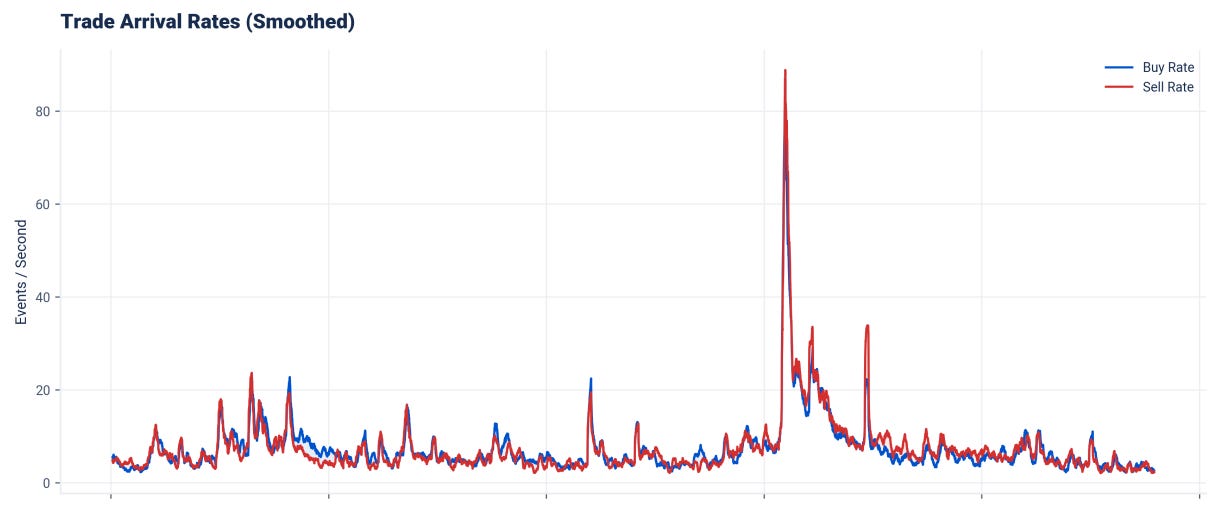
In this article, we will be exploring models that are able to capture those phenomena and use them to model order-flow, a very important metric to keep an eye on in high-frequency trading!

Full Code available at the End!

---

Table of Contents

1. Point Process — The Mathematics of Random Events

2. Poisson Process — Why the Textbook Model Fails

3. Poisson-GLM and Binned Intensities — Smarter Order-Flow Model

4. Hawkes Process — When Past Trades Trigger Future Trades

5. Multivariate Hawkes Process — How Buys Excite Sells (and Vice Versa)

6. Extensions and Conclusion — Extensions, Final Remarks and Discord

---

Point Process — The Mathematics of Random Events

At its core, a point process is a random collection of points in some space, in our case, time. A point process in space could be where a raindrop hits the ground, for example. When modelling Order-Flow, each event happens at a specific time, and the pattern of these occurrences is random rather than deterministic.

Formally, a point process N on a space S is a random countable collection of points. For any measurable set A ⊆ S, the quantity N(A) represents the (random) number of points falling within A.

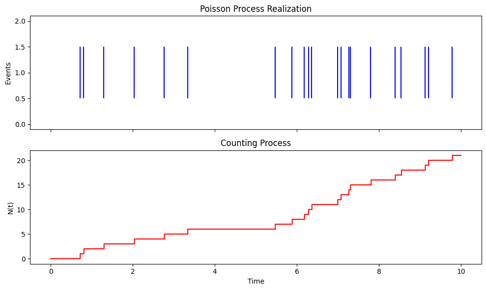
Counting Process Representation

When working with point processes in time (S = [0, ∞)), we often use the counting process representation. Define N(t) as the number of events that have occurred in the interval [0, t]:

\(N(t) = \sum_{i=1}^{\infty} 1_{\{T_i \leq t\}}\)

where T_1, T_2, … are random arrival times of events with 0 < T_1 < T_2 < ….
The function N(t) is non-decreasing, right-continuous, and takes integer values, jumping by 1 at each arrival time.

Here is one example of a realisation of a point process and the corresponding counting process representation:

Key Characteristics

There are several quantities that characterise the behaviour of a point process. Consider, for example, the following 2 point process realisations:

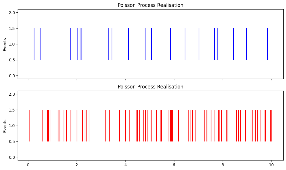
Right off the bat, you can tell that the second one seems to be more intense, whatever that means.

The so-called intensity function described the instantaneous rate at which events occur:

\(\lambda(t) = \lim_{\Delta t \to 0} \frac{E[N(t+ \Delta t) - N(t)]}{\Delta t}\)

This captures the expected number of events per unit time in an infinitesimal interval after t. For many point processes, we can write the expected number of points in an interval [a,b] as:

\(E[N(b)-N(a)] = \int_a^b\lambda(s)ds\)

The conditional intensity provides even more information by incorporating the history of the process up to time t:

\(\lambda(t|\mathcal{F}_t) = \lim_{\Delta t \to 0} \frac{\mathbb{P}(N(t+\Delta t) - N(t) = 1 | \mathcal{F}_t)}{\Delta t}\)

with respect to a filtration F_t. You can imagine F_t as the history of events preceding time t. If you need to catch up on filtrations, I recommend that you check out the following article:

Option Pricing Basics

I explain Filtrations intuitively there.