How to Price Touch-Style Options (Polymarket)

And how to profit from mispricings

“What price will Bitcoin hit in November?”. This is one of many markets on Polymarket that allows you to speculate on the price of Cryptocurrencies.

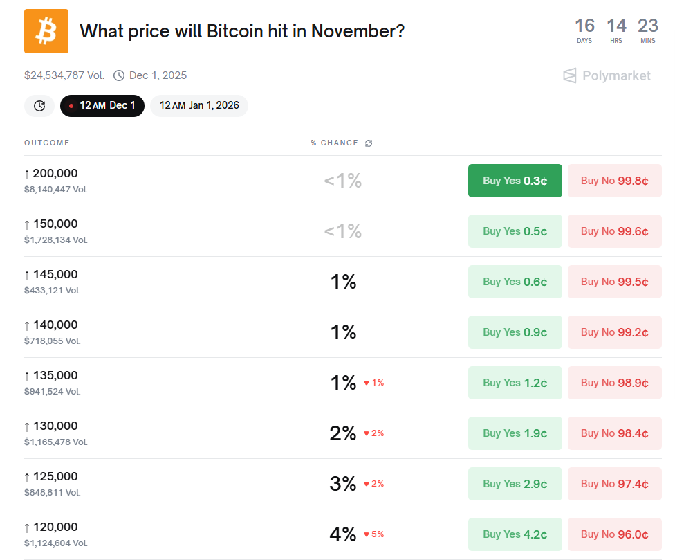
What you see in this picture are essentially options contracts!
You can buy a share of “Bitcoin price will be above $130.000 at some point in November” for 1.9 Cents, and if this ends up happening, you will receive $1.0, a profit of $0.981. You can also bet that it won’t happen for the price of $98.4. Both Yes and No have their own order book.

What we will do in this article is price those options using data from a larger options market, Deribit.
We do this because, on average, a bigger and more liquid option market will better reflect fair prices. If Polymarket prices are way out of line with what Deribit implies, then that’s an opportunity to profit!

---

Setting Up the Environment

Before we can get started pricing those options, let us first set up our environment. This means importing libraries and defining important variables:

import numpy as np
import pandas as pd
import math
import json
import os
import re
import time
import urllib.error
import urllib.parse
import urllib.request
from typing import Optional, Tuple, Dict, List
from datetime import datetime, timezone

import matplotlib.pyplot as plt
from matplotlib.ticker import FuncFormatter
from matplotlib import cm
from scipy.interpolate import PchipInterpolator, RegularGridInterpolator
from scipy.stats import gaussian_kde, norm
from scipy.optimize import least_squares

print(”Dependencies ready.”)

Here are all of the libraries we are gonna be using in this article. If you don’t have any of them, you can install them via

pip install *library name*

Now our parameters:

# User-editable parameters


# --- Core asset / horizon ---
UNDERLYING = “BTC”                  # “BTC” or “ETH”
EXPIRY_ISO = “2026-01-01”           # Target option/barrier horizon (YYYY-MM-DD)
VALUATION_DT = None                  # None = now (UTC) ; or “YYYY-MM-DD HH:MM” (local)

# --- Monte Carlo config ---
N_PATHS_HIT = 200_000               # Hit probability estimation & sweep envelopes
N_STEPS = None                      # None = ~daily; or set an int
SEED = 42                           # Reproducibility seed used everywhere
MBTCOD = “bb”                       # ‘bb’ (bridge), ‘gobet’, or ‘bb_gobet’
USE_MID_SIGMA = True                # Use mid-step sigma in bridge/shift

# --- K sweep ---
SWEEP_POINTS = 301                  # Number of K points across the grid
S_MIN_FACTOR = 0.25                 # Grid min = factor * spot
S_MAX_FACTOR = 3.00                 # Grid max = factor * spot

# --- Gating (Polymarket comparison) ---
ABS_THRESHOLD = 0.03                # Must exceed both CI margin and this absolute threshold

# --- Output locations ---
BASE_DIR = os.getcwd()
SNAPSHOT_DIR = os.path.join(BASE_DIR, “data_snapshots”)
SMILES_DIR = os.path.join(BASE_DIR, “smiles_term_structure”)
OUTPUTS_DIR = os.path.join(BASE_DIR, “outputs”)

# Output filenames (lowercase for convenience)
EXP_STR = EXPIRY_ISO.replace(”-”, “”)
SWEEP_CSV = os.path.join(OUTPUTS_DIR, f”{UNDERLYING.lower()}_probability_sweep.csv”)
META_JSON = os.path.join(OUTPUTS_DIR, f”{UNDERLYING.lower()}_probability_sweep_meta.json”)
PLOT_PNG = os.path.join(OUTPUTS_DIR, f”polymarket_vs_model_{UNDERLYING.lower()}_{EXP_STR}.png”)

# Ensure directories
os.makedirs(SNAPSHOT_DIR, exist_ok=True)
os.makedirs(SMILES_DIR, exist_ok=True)
os.makedirs(OUTPUTS_DIR, exist_ok=True)

print(”Parameters set.”)

Some of those should be pretty self-explanatory. The other ones, like the “K sweep” parameters, will be popping up in the code in later chapters.

---

Data Retrieval

We can’t price anything without data. This section of the article will be all about gathering all of the data we need and putting it into a nice format.

Helpers

First, some useful utilities:

def yearfrac_365(start: datetime, end: datetime) -> float:
    return max(0.0, (end - start).total_seconds() / (365.25 * 24 * 3600.0))

This function tells us how many years are between start and end, which are both datetime objects.

def fetch_url_text(url: str, timeout: float = 10.0) -> Optional[str]:
    try:
        with urllib.request.urlopen(url, timeout=timeout) as resp:
            return resp.read().decode(”utf-8”)
    except Exception:
        return None

This function makes a request to the given URL and returns the text of the response.

Risk-free Rates

Option prices depend on risk-free rates, because an option’s payoff can be replicated using the underlying asset and a risk-free bond, and this risk-free bond’s price depends on the risk-free rate.

Under risk-neutral valuation, we have:

\(\text{Option Price} = e^{-rT}E[\text{Payoff}]\)

where the expectation is under risk-neutral probabilities.
To learn more about general option pricing like this, check out my dedicated article:

We can grab the latest yearly interest rate directly from FRED.
By default, we will use the Secured Overnight Financing Rate (SOFR), the most common benchmark for risk-free rates in the US. Our fallback will be the 3-Month Treasury Yield (DGS3MO), the interest on a 3-month US Treasury Bill.

Here is the function to grab those from FRED:

def fetch_fred_latest(series_id: str) -> Optional[float]:
    “”“Fetch latest non-missing value from FRED (percent -> decimal).”“”
    url = f”https://fred.stlouisfed.org/graph/fredgraph.csv?id={series_id}”
    txt = fetch_url_text(url, timeout=10)
    if not txt:
        return None
    lines = [ln.strip() for ln in txt.splitlines() if ln.strip()]
    for ln in reversed(lines[1:]):  # skip header
        parts = ln.split(”,”)
        if len(parts) < 2:
            continue
        val = parts[1].strip()
        if val not in (”.”, “”, “NaN”):
            try:
                return float(val) / 100.0
            except ValueError:
                continue
    return None

It’s more convenient to work with continuous interest rates rather than simple annual interest rates.

For the simple annual interest rate R, we have that $1 in T years is worth:

\(\text{Value} = 1 + RT\)

While for a continuous interest rate r, we have that $1 in T years is worth:

\(\text{Value} = e^{rT}\)

If we ask ourselves the opposite question (What is $1 in T years worth today?), we get the so-called “discount factor”, which for the simple linear interest rate is:

\(\text{df} = \frac{1}{1+RT}\)

and for the continuous interest rate:

\(df = e^{-rT}\)

We can equate those two and solve for r to be able to convert linear interest rates to continuous ones:

\(r = \frac{\ln(1+RT)}{T} = -\frac{\ln (\text{df})}{T}\)

Here is the code that does that:

def simple_to_cc(y_simple: float, T_years: float, daycount_base: float, quote_base: float) -> float:
    “”“
    Convert a simple annualized rate (quoted on quote_base) to continuous compounding over T_years.
    df = 1 / (1 + y_simple * T_quote) with T_quote = T_years * (daycount/quote); r_cc = -ln(df) / T_years
    “”“
    T_quote = T_years * (daycount_base / quote_base)
    df = 1.0 / max(1e-12, 1.0 + y_simple * T_quote)
    return -math.log(df) / max(T_years, 1e-12)

Note: This code looks a little more complicated than what we just described. The reason for this is that different sources of interest rates use different definitions of what a year is. Some use 360 days, while others use 365 days, etc. This code automatically accounts for that.

Finally, we can combine all those functions into one function that will give us our continuous risk-free rate with a simple function call:

def get_risk_free_cc(T: float) -> Tuple[float, Dict[str, float]]:
    “”“
    Compute continuous-comp risk-free over T years.
    Preferred: SOFR (ACT/360) -> CC. Fallback: DGS3MO (approx ACT/365) -> CC.
    “”“
    meta = {”source”: “”, “raw_rate”: np.nan}
    sofr = fetch_fred_latest(”SOFR”)
    if sofr is not None and sofr > 0.0:
        r = simple_to_cc(y_simple=sofr, T_years=T, daycount_base=365.25, quote_base=360.0)
        meta.update({”source”: “SOFR (FRED)”, “raw_rate”: sofr})
        return float(r), meta
    tbill3m = fetch_fred_latest(”DGS3MO”)
    if tbill3m is not None and tbill3m > 0.0:
        r = simple_to_cc(y_simple=tbill3m, T_years=T, daycount_base=365.25, quote_base=365.25)
        meta.update({”source”: “DGS3MO (FRED)”, “raw_rate”: tbill3m})
        return float(r), meta
    meta.update({”source”: “fallback_zero”, “raw_rate”: 0.0})
    return 0.0, meta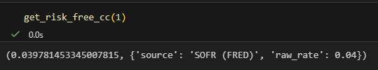

Spot, Futures, and Carry

We also need spot and futures prices to compute carry. We will use Binance as our standard and Deribit as a fallback.

First, we have some simple helpers that make our life a little easier:

def http_get_json(url: str, timeout: float = 10.0) -> Optional[dict]:
    txt = fetch_url_text(url, timeout=timeout)
    if not txt:
        return None
    try:
        return json.loads(txt)
    except Exception:
        return None

This function makes a request to the given URL and returns the JSON.

def deribit_api(path: str, params: Dict[str, str]) -> Optional[dict]:
    q = urllib.parse.urlencode(params)
    url = f”{DERIBIT_BASE}{path}?{q}”
    try:
        with urllib.request.urlopen(url, timeout=10) as resp:
            data = json.loads(resp.read().decode(”utf-8”))
            if data.get(”result”) is not None:
                return data[”result”]
            return None
    except Exception:
        return None

This function simplifies calling the Deribit API.

Next are 2 functions for getting the Binance and Deribit Spot price for a given underlying:

def fetch_spot_binance(underlying: str) -> Optional[float]:
    symbol = {”BTC”: “BTCUSDT”, “ETH”: “ETHUSDT”}.get(underlying.upper())
    if not symbol:
        return None
    url = f”https://api.binance.com/api/v3/ticker/price?symbol={symbol}”
    try:
        with urllib.request.urlopen(url, timeout=10) as resp:
            data = json.loads(resp.read().decode(”utf-8”))
            return float(data[”price”]) if “price” in data else None
    except Exception:
        return None


def fetch_spot_fallback_deribit(underlying: str) -> Optional[float]:
    # Deribit index price for BTC/ETH in USD
    index_name = “btc_usd” if underlying.upper() == “BTC” else “eth_usd”
    res = deribit_api(”public/get_index_price”, {”index_name”: index_name})
    if res and “index_price” in res:
        return float(res[”index_price”])
    return None

As I said before, we want to use Binance as a default and Deribit as a fallback. The following function does this for us:

def fetch_spot(underlying: str) -> Optional[float]:
    px = fetch_spot_binance(underlying)
    if px is not None:
        return px
    return fetch_spot_fallback_deribit(underlying)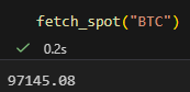

Now that we can grab spot prices, let’s move on to futures. We will use Deribit to get Futures and Option prices, as Deribit is the go-to exchange for those dated derivatives and has by far the highest liquidity and open interest.

The following function will return all non-perp futures on Deribit for the given underlying:

def deribit_fetch_futures(currency: str) -> Optional[List[dict]]:
    res = deribit_api(”public/get_instruments”, {”currency”: currency, “kind”: “future”, “expired”: “false”})
    if not res:
        return None
    return [x for x in res if not x.get(”is_perpetual”, False)]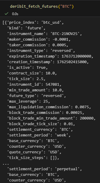

The following function will compute the midprice for a given instrument:

def deribit_ticker_mid(instrument_name: str) -> Optional[float]:
    res = deribit_api(”public/ticker”, {”instrument_name”: instrument_name})
    if not res:
        return None
    bid = res.get(”best_bid_price”) or res.get(”bid_price”)
    ask = res.get(”best_ask_price”) or res.get(”ask_price”)
    mark = res.get(”mark_price”)
    last = res.get(”last_price”)
    if bid and ask and bid > 0 and ask > 0:
        return 0.5 * (bid + ask)
    if mark and mark > 0:
        return float(mark)
    if last and last > 0:
        return float(last)
    return None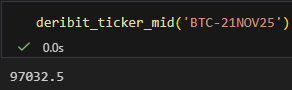

If we can’t get the midprice, we will fall back to the mark price. If that doesn’t work, our last resort is the last traded price.

Why do we even need spot and futures prices? The reason is Carry.
Carry is the cost of keeping a financial position open if the price doesn’t move.
Cost here doesn’t just mean pure P&L. We could have $2 P&L, but if we could have made $5 risk-free instead, then making 2 bucks isn’t all that great.

We can extract the implied carry from the standard futures pricing model:

\(F=Se^{cT}\)

where F is the futures price, S is the spot price, c is carry, and T is the time to maturity.

Solving for c, we obtain:

\(c = \frac{\ln(\frac{F}{S})}{T}\)

If we want the carry implied by a future with maturity of 0.5 years, but we only have futures with maturities of 0.3 years and 0.6 years, then we can calculate the carry for both and interpolate linearly. The following function computes carries and handles everything like requesting prices and interpolating for us:

def compute_carry_from_deribit(spot: float, valuation_dt: datetime, target_T: float, currency: str) -> Tuple[Optional[float], Dict]:
    meta = {”source”: “Deribit”, “used”: [], “interpolation”: “”}
    insts = deribit_fetch_futures(currency)
    if not insts:
        return None, meta
    now_ts = valuation_dt.replace(tzinfo=timezone.utc).timestamp()
    pts = []
    for x in insts:
        exp_ms = x.get(”expiration_timestamp”)
        name = x.get(”instrument_name”)
        if not exp_ms or not name:
            continue
        exp_ts = exp_ms / 1000.0
        T_i = max(0.0, (exp_ts - now_ts) / (365.25 * 24 * 3600.0))
        if T_i <= 1e-6:
            continue
        mid = deribit_ticker_mid(name)
        if not mid or mid <= 0:
            continue
        c_i = math.log(mid / spot) / T_i
        pts.append((T_i, c_i, name))
    if not pts:
        return None, meta
    pts.sort(key=lambda z: z[0])
    lower = None
    upper = None
    for T_i, c_i, name in pts:
        if T_i < target_T:
            lower = (T_i, c_i, name)
        elif T_i >= target_T and upper is None:
            upper = (T_i, c_i, name)
    if lower and upper and upper[0] > lower[0] + 1e-12:
        Tl, cl, nl = lower
        Th, ch, nh = upper
        w = (target_T - Tl) / (Th - Tl)
        c_T = cl + (ch - cl) * w
        meta[”used”] = [{”instrument”: nl, “T”: Tl, “carry”: cl}, {”instrument”: nh, “T”: Th, “carry”: ch}]
        meta[”interpolation”] = “linear”
        return c_T, meta
    Tn, cn, nn = min(pts, key=lambda z: abs(z[0] - target_T))
    meta[”used”] = [{”instrument”: nn, “T”: Tn, “carry”: cn}]
    meta[”interpolation”] = “nearest”
    return cn, meta

We can break carry up into 2 components, risk-free rate and other cashflow like dividends, staking, etc.:

\(c = r-q\)

The following function will compute this q from carry and the risk-free rate:

def get_rates_auto(spot: float, valuation_dt: datetime, expiry_dt: datetime, currency: str) -> Tuple[float, float, Dict]:
    T = yearfrac_365(valuation_dt, expiry_dt)
    r_cc, r_meta = get_risk_free_cc(T)
    c_T, c_meta = compute_carry_from_deribit(spot, valuation_dt, T, currency)
    meta = {
        “r_source”: r_meta.get(”source”, “”),
        “r_raw_rate”: r_meta.get(”raw_rate”, np.nan),
        “c_source”: c_meta.get(”source”, “Deribit”),
        “c_meta”: c_meta,
        “T_years”: T,
    }
    if c_T is None:
        q = 0.0
        meta[”note”] = “Futures basis unavailable; funding set to 0.0”
        return r_cc, q, meta
    q = r_cc - c_T
    return r_cc, float(q), meta

Options

Let’s move on to the last part of data gathering: Option prices and Implied Volatilities.

The following function will grab all live option on Deribit:

def deribit_fetch_option_instruments(currency: str) -> Optional[List[dict]]:
    res = deribit_api(”public/get_instruments”, {”currency”: currency, “kind”: “option”, “expired”: “false”})
    if not res:
        return None
    return res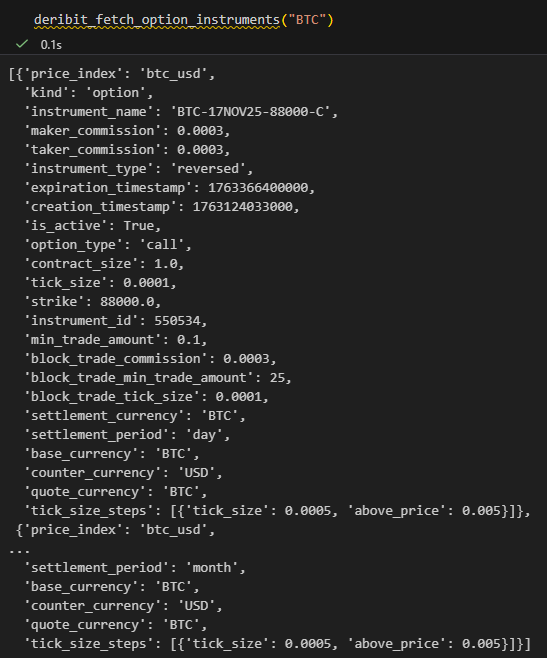

Just like in the futures situation, we only have a finite number of expiries for options.

For a given target expiry, the following function will give us the closest available expiries actually available:

def select_expiries_around_target(option_instruments: List[dict], target_dt: datetime, max_expiries: int = 6) -> List[datetime]:
    # Collect unique expiry datetimes
    exps_ms = sorted(set(int(x[”expiration_timestamp”]) for x in option_instruments if x.get(”expiration_timestamp”)))
    exps_dt = [datetime.utcfromtimestamp(ms / 1000.0) for ms in exps_ms]
    if not exps_dt:
        return []
    # Rank by distance to target, ensure at least one below and above if possible
    exps_sorted = sorted(exps_dt, key=lambda d: abs((d - target_dt).total_seconds()))
    chosen = []
    for d in exps_sorted:
        if d not in chosen:
            chosen.append(d)
        if len(chosen) >= max_expiries:
            break
    # Sort ascending
    chosen = sorted(chosen)
    return chosen

For each of those expiries, we can grab all available options and return their implied volatilities. The following function returns a dataframe of all those volatility smiles:

def build_smiles_for_expiries(currency: str, chosen_expiries: List[datetime]) -> Dict[str, pd.DataFrame]:
    “”“
    For each expiry, fetch all option tickers and extract ‘mark_iv’ by strike.
    Returns a dict: expiry_iso -> DataFrame with columns [’Strike’,’Implied Volatility’,’Expiry’].
    ‘Implied Volatility’ in percent for easier CSV inspection.
    “”“
    insts = deribit_fetch_option_instruments(currency)
    if not insts:
        return {}
    # Bucket instruments by expiry
    buckets: Dict[int, List[dict]] = {}
    for x in insts:
        exp_ms = x.get(”expiration_timestamp”)
        strike = x.get(”strike”)
        if not exp_ms or strike is None:
            continue
        buckets.setdefault(exp_ms, []).append(x)

    smiles: Dict[str, pd.DataFrame] = {}
    for exp_dt in chosen_expiries:
        exp_ms = int(exp_dt.replace(tzinfo=timezone.utc).timestamp() * 1000)
        group = buckets.get(exp_ms, [])
        rows = []
        for inst in group:
            name = inst.get(”instrument_name”)
            strike = inst.get(”strike”)
            if not name or strike is None:
                continue
            tick = deribit_api(”public/ticker”, {”instrument_name”: name})
            if not tick:
                continue
            mark_iv = tick.get(”mark_iv”)
            if mark_iv is None or mark_iv <= 0:
                continue
            iv_val = float(mark_iv)
            iv_pct = iv_val * 100.0 if iv_val <= 1.5 else iv_val
            rows.append({”Strike”: float(strike), “Implied Volatility”: iv_pct})
        if not rows:
            continue
        df = pd.DataFrame(rows).dropna().drop_duplicates(”Strike”).sort_values(”Strike”)
        df[”Expiry”] = exp_dt.strftime(”%Y-%m-%d”)
        smiles[df[”Expiry”].iloc[0]] = df
    return smiles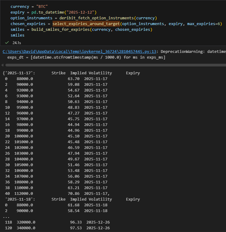

---

SVI Model fitting

We are finally done with all the prerequisite work. Let’s move on to the fun part of modelling! There are a few problems with using raw option prices for a volatility smile: