
Looking Inside The Black Box
Model-agnostic interpretable machine learning

People often criticise how ML models are just black boxes that take in some features and spit out a prediction. While some models (like linear regression) are naturally a lot more interpretable than others (like neural networks), it’s wrong that you can’t figure out why a model made a certain prediction and how the different features affect the prediction.
In this article, we will look at some useful model-agnostic methods (meaning that it doesn’t matter what model we apply it to) for figuring out why one specific prediction is what it is (Local Methods) and why predictions are what they are on average (Global Methods).
This is important for a few very important reasons.
Detecting problems in the model:
Say you built a model that forecasts raw returns, and you see that the error has a lower error than some baseline model. A lot of people would quit here, but you dig deeper and find out that the only feature that matters to the model is volatility, and that the only thing that the model learned to do well is predict the magnitude of the return, not the sign. Suddenly, the model is completely useless for what it was supposed to do!Regulatory & risk management requirements:
Regulators increasingly require that automated trading and risk models be explainable. If your model flags a position as too risky or generates a trade signal, compliance needs to know why. A black box doesn’t pass that bar.
Detecting data leakage:
If your model is suspiciously good, interpretability tells you what it’s actually learning. Example: a return-prediction model that learned to exploit a look-ahead bias in a feature, e.g., using end-of-day prices to predict intraday moves, shows up immediately as one feature with overwhelming importance.
Feature engineering feedback loop:
Once you know which features are actually driving predictions, you can iterate intelligently; drop redundant factors, identify which alpha signals are being ignored, or understand why a signal that worked in research is being suppressed by the model in production.
Regime analysis:
Local methods let you compare why the model made a prediction in a bull market vs. a crisis period. If the feature importances shift dramatically across regimes, that’s a red flag for out-of-sample robustness; your model may have overfit to one regime’s dynamics.
More interpretable models are often less accurate, and model-agnostic post-hoc methods let you have both: full model flexibility and explanations.
I write about quantitative trading the way it’s actually practiced:
Robust models and portfolios, combining signals and strategies, understanding the assumptions behind your models.
More broadly, I write about:
Statistical and cross-sectional arbitrage
Managing multiple strategies and signals
Risk and capital allocation
Research tooling and methodology
In-depth model assumptions and derivations
If this way of thinking resonates, you’ll probably like what I publish.
1. Local Model-agnostic Methods
Local methods answer a specific question: why did the model predict this value for this observation? Rather than summarising model behaviour across the entire dataset, they explain a single prediction by attributing it to the input features of that one data point.
Example: Your model predicts a large positive return for a particular asset on a particular day. A global method might tell you that momentum is generally the most important feature in your model. But a local method tells you that for this specific prediction, the signal was driven almost entirely by a spike in order flow imbalance, while momentum actually pushed the prediction slightly lower. That distinction matters enormously when you're trying to understand a model's live behaviour, debug an unexpected signal, or explain a specific trade to a risk committee.
Let’s go over some of the most popular methods.
1.1 Ceteris Paribus Plots
The name sounds really complicated, but it’s actually the simplest method you could use. Ceteris Paribus is Latin for "all other things being equal". As the name implies, to analyze a certain feature, you simply change its value while keeping all other features unchanged and look at the resulting predictions.
Before looking more into this method, let us train a model that we will keep using as an example for all methods. We will do a 1-day-ahead prediction of SPY returns using some basic features like momentum, RSI, etc. Doesn’t matter if the model is garbage as long as we can run our analysis on it.
First we load our data:
import pandas as pd
import numpy as np
import matplotlib.pyplot as plt
import yfinance as yf
def load_spy():
df = yf.download("SPY", start="2010-01-01", end="2026-03-27", auto_adjust=True)
df.columns = df.columns.droplevel(1)
df["ret"] = df["Close"].pct_change()
df["target"] = df["ret"].shift(-1) # next-day return
# Momentum
df["mom_5"] = df["ret"].rolling(5).mean()
df["mom_20"] = df["ret"].rolling(20).mean()
df["mom_60"] = df["ret"].rolling(60).mean()
# Volatility
df["vol_5"] = df["ret"].rolling(5).std()
df["vol_20"] = df["ret"].rolling(20).std()
df["vol_ratio"] = df["vol_5"] / df["vol_20"] # vol regime indicator
# Mean reversion
df["rsi_14"] = _rsi(df["Close"], 14)
df["zscore_20"] = (df["Close"] - df["Close"].rolling(20).mean()) / df["Close"].rolling(20).std()
# Volume
df["volume_z"] = (df["Volume"] - df["Volume"].rolling(20).mean()) / df["Volume"].rolling(20).std()
# Price-based
df["hl_range"] = (df["High"] - df["Low"]) / df["Close"] # normalized daily range
df["gap"] = (df["Open"] - df["Close"].shift(1)) / df["Close"].shift(1) # overnight gap
# Autocorrelation signal
df["ret_lag1"] = df["ret"].shift(1)
df["ret_lag2"] = df["ret"].shift(2)
features = [
"mom_5", "mom_20", "mom_60",
"vol_5", "vol_20", "vol_ratio",
"rsi_14", "zscore_20",
"volume_z", "hl_range", "gap",
"ret_lag1", "ret_lag2"
]
df = df[["target"] + features].dropna()
return df
def _rsi(close, period=14):
delta = close.diff()
gain = delta.clip(lower=0).rolling(period).mean()
loss = (-delta.clip(upper=0)).rolling(period).mean()
rs = gain / loss
return 100 - (100 / (1 + rs))df = load_spy()
df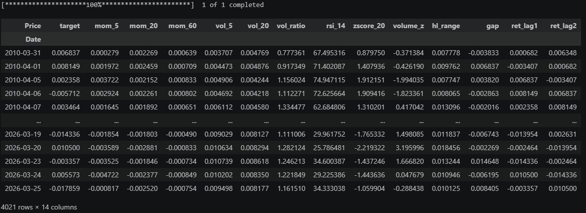
And now let’s train an XGBoost model to predict the next day’s return using our features (We won’t be doing any train-test splits or other important steps here, this is purely an exercise model!):
from xgboost import XGBRegressor
from sklearn.metrics import r2_score
FEATURES = [c for c in df.columns if c != "target"]
X = df[FEATURES]
y = df["target"]
model = XGBRegressor(n_estimators=300, max_depth=4, learning_rate=0.05,
subsample=0.8, colsample_bytree=0.8, random_state=42)
model.fit(X, y)preds = model.predict(X)
df["forecast"] = preds
df[["target", "forecast"]].to_csv("forecasts.csv")Price target forecast
Date
2010-03-31 0.006837 0.000646
2010-04-01 0.008149 0.000556
2010-04-05 0.002358 -0.000046
2010-04-06 -0.005712 0.000146
2010-04-07 0.003464 0.001303Back to Ceteris Paribus.
Here is an implementation of it:
def cp_profile(model, X, obs_idx, feature, n_points=100):
    x_obs = X.iloc[[obs_idx]].copy()
    grid = np.linspace(X[feature].min(), X[feature].max(), n_points)
    preds = []
    for val in grid:
        x_obs[feature] = val
        preds.append(model.predict(x_obs)[0])
    return grid, np.array(preds)
Let’s try it on the 2026-03-03 prediction for the features "mom_20", "vol_20", "rsi_14", "zscore_20":
Price
target        0.007055
mom_5        -0.002033
mom_20       -0.001063
mom_60       -0.000015
vol_5         0.006754
vol_20        0.008314
vol_ratio     0.812388
rsi_14       39.089484
zscore_20    -1.367428
volume_z      1.027870
hl_range      0.019035
gap          -0.016492
ret_lag1      0.000569
ret_lag2     -0.004802
forecast      0.001172
Name: 2026-03-03 00:00:00, dtype: float64
obs_idx = X.index.get_loc("2026-03-03")
features_to_plot = ["mom_20", "vol_20", "rsi_14", "zscore_20"]
fig, axes = plt.subplots(len(features_to_plot), 1, figsize=(9, 14))
fig.suptitle("Ceteris Paribus Profiles — SPY XGBoost (2026-03-01)", fontsize=14, fontweight="bold")
for ax, feat in zip(axes, features_to_plot):
grid, preds = cp_profile(model, X, obs_idx, feat)
ax.plot(grid, preds, linewidth=1.8)
ax.axvline(X.iloc[obs_idx][feat], color="red", linestyle="--", label="observed value")
ax.axhline(0, color="black", linewidth=0.8, linestyle="--")
ax.set_xlabel(feat, fontsize=11)
ax.set_ylabel("Predicted return", fontsize=10)
ax.legend(fontsize=9)
ax.grid(True, alpha=0.3)
plt.tight_layout()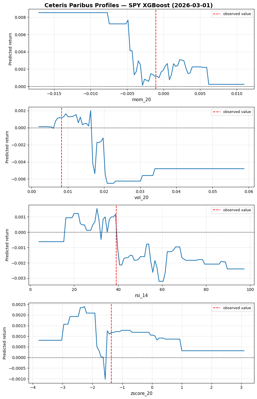
If momentum were even more negative, we would have predicted an even more positive return (mean reversion effect). If volatility were higher, we would have flipped to strongly negative instead (flipping from mean reversion to momentum).
Many of the methods we will look at are creative combinations of multiple Ceteris Paribus plots that tell us more.
The BIG problem with this (and many other) methods is correlation among features.
Changing one feature while keeping the others unchanged can give us unrealistic feature combinations, like huge recent momentum while volatility is very low.
1.2 Individual Conditional Expectation (ICE)
An ICE plot is simply many Ceteris Paribus plots overlaid, one per observation.
Here is an implementation:
def ice_plot(model, X, feature, n_obs=100, n_points=100):
    sample = X.sample(n_obs, random_state=42)
    grid = np.linspace(X[feature].min(), X[feature].max(), n_points)

    fig, ax = plt.subplots(figsize=(9, 4))
    for idx in range(len(sample)):
        _, preds = cp_profile(model, sample.reset_index(drop=True), idx, feature, n_points)
        ax.plot(grid, preds, color="steelblue", alpha=0.4, linewidth=0.8)

    ax.axhline(0, color="black", linewidth=0.8, linestyle="--")
    ax.set_xlabel(feature)
    ax.set_ylabel("Predicted return")
    ax.grid(True, alpha=0.3)
    plt.title(f"ICE Plot — {feature}")
    plt.tight_layout()
Let’s run it for “mom_20”:
ice_plot(model, X, "mom_20")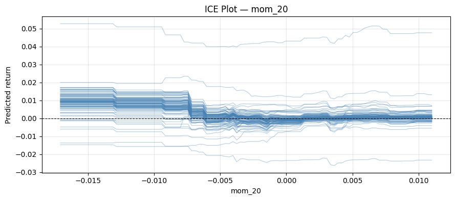
We can explore interactions with this method by using colors.
def ice_plot(model, X, feature, color_by=None, n_obs=100, n_points=100):
    sample = X.sample(n_obs, random_state=42).reset_index(drop=True)
    grid = np.linspace(X[feature].quantile(0.01), X[feature].quantile(0.99), n_points)

    fig, ax = plt.subplots(figsize=(9, 4))
    for idx in range(len(sample)):
        _, preds = cp_profile(model, sample, idx, feature, n_points)
        if color_by is not None:
            median = sample[color_by].median()
            color = "#d62728" if sample[color_by].iloc[idx] > median else "#1f77b4"
        else:
            color = "steelblue"
        ax.plot(grid, preds, color=color, alpha=0.4, linewidth=0.8)

    if color_by is not None:
        ax.plot([], [], color="#d62728", label=f"{color_by} high")
        ax.plot([], [], color="#1f77b4", label=f"{color_by} low")
        ax.legend(fontsize=9)

    ax.axhline(0, color="black", linewidth=0.8, linestyle="--")
    ax.set_xlabel(feature)
    ax.set_ylabel("Predicted return")
    ax.grid(True, alpha=0.3)
    plt.title(f"ICE Plot — {feature}" + (f" | colored by {color_by}" if color_by else ""))
    plt.tight_layout()
Let’s color in low/high volatility:
ice_plot(model, X, "mom_20", "vol_20")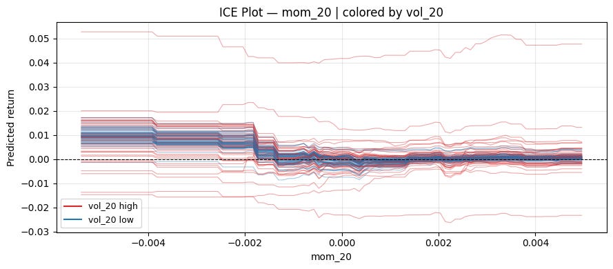
Centered ICE Plot:
It can be hard to tell if the different curves are affected equally by the feature of interest because they have different levels.
A simple solution is to subtract each curve's value at some specific value of x. This removes the vertical spread caused by other features and lets you focus purely on the effect of varying the feature of interest.
def cp_profile(model, X, obs_idx, feature, grid):
    x_obs = X.iloc[[obs_idx]].copy()
    preds = [model.predict(x_obs.assign(**{feature: val}))[0] for val in grid]
    return np.array(preds)

def ice_plot(model, X, feature, color_by=None, centered=False, ref_value=None, n_obs=100, n_points=100):
    sample = X.sample(n_obs, random_state=42).reset_index(drop=True)
    grid = np.linspace(X[feature].quantile(0.01), X[feature].quantile(0.99), n_points)
    if centered and ref_value is not None:
        grid = np.sort(np.append(grid, ref_value))  # ensure ref_value is exactly in grid

    fig, ax = plt.subplots(figsize=(9, 4))
    for idx in range(len(sample)):
        preds = cp_profile(model, sample, idx, feature, grid)
        if centered:
            ref = ref_value if ref_value is not None else grid[0]
            ref_pred = preds[np.searchsorted(grid, ref)]
            preds = preds - ref_pred
        color = "steelblue"
        if color_by is not None:
            color = "#d62728" if sample[color_by].iloc[idx] > sample[color_by].median() else "#1f77b4"
        ax.plot(grid, preds, color=color, alpha=0.3, linewidth=0.8)

    if color_by is not None:
        ax.plot([], [], color="#d62728", label=f"{color_by} high")
        ax.plot([], [], color="#1f77b4", label=f"{color_by} low")
        ax.legend(fontsize=9)

    ax.axhline(0, color="black", linewidth=0.8, linestyle="--")
    ax.set_xlabel(feature)
    ax.set_ylabel("Change in predicted return" if centered else "Predicted return")
    ax.grid(True, alpha=0.3)
    plt.title(f"{'c-ICE' if centered else 'ICE'} Plot — {feature}" + (f" | colored by {color_by}" if color_by else ""))
    plt.tight_layout()
A natural reference point for momentum is 0:
ice_plot(model, X, "mom_20", "vol_20", centered=True, ref_value=0)
Can see a pretty clear pattern on the left! When volatility is high, momentum works. When volatility is low, mean reversion works.
1.3 Local interpretable model-agnostic explanations (LIME)
CP profiles and ICE show you how the prediction changes as you vary one feature. But they don’t give you a single number answering: how much did feature x contribute to this specific prediction? LIME does exactly that.
The basic idea is that our black box method f is too complex to interpret globally, so we interpret near a specific observation x (all our features at one specific date) by training a simpler model (for example linear) in a small neighborhood of x.
Here is how LIME does this exactly (using linear regression as an example for the interpretable model):
Perturbing the observation:
Generate N synthetic samples by randomly perturbing the features around x. For tabular data, this is done by sampling each feature from its marginal distribution. For continuous data, this is done by sampling from a normal distribution with equal means and standard deviations to the training set (This again ignores correlations! A typical weakness of LIME).Weighing by proximity:
Each synthetic sample z is weighted by how close it is to x using an exponential kernel:\(\pi_x(z) = \exp(-\frac{d(x,z)^2}{\sigma^2})\)In our case, d will be euclidian distance, but other measures of distance can be chosen too.
Fitting a weighted linear model:
Run the black-box model on all synthetic samples to get labels, then fit a weighted linear regression:\(\hat{g} = \arg \min_g \sum_z \pi_x(z) (\hat{f}(z) - g(z))^2\)Reading the explanation:
Now we interpret the resulting model. In the case of linear regression, that’s easy, as we simply look at the coefficients.
Let’s implement this with ridge regression, which handles our correlated features better:
def lime_explain(model, X, obs_idx, n_samples=1000, sigma=1.0, ridge_alpha=1.0):
    x_obs = X.iloc[obs_idx].values
    means = X.mean().values
    stds  = X.std().values

    # 1. perturb
    Z = np.random.normal(means, stds, size=(n_samples, X.shape[1]))

    # 2. weights
    Z_std = (Z - x_obs) / stds
    distances = np.sqrt((Z_std ** 2).sum(axis=1))
    weights = np.exp(-distances ** 2 / sigma ** 2)

    # 3. black-box labels
    labels = model.predict(Z)

    # 4. fit weighted linear model
    lr = Ridge(alpha=ridge_alpha)
    lr.fit(Z, labels, sample_weight=weights)

    return dict(zip(X.columns, lr.coef_))
And run it again for our 2026-03-03 forecast:
obs_idx = X.index.get_loc("2026-03-03")
explanation = lime_explain(model, X, obs_idx)
print(explanation)
mom_5 -2.096855e-09
mom_20 -4.942316e-09
mom_60 4.846428e-09
vol_5 4.087705e-08
vol_20 1.238100e-08
vol_ratio 5.578009e-07
rsi_14 -1.130377e-05
zscore_20 -2.909305e-06
volume_z -1.143078e-06
hl_range -4.011315e-08
gap 2.016699e-08
ret_lag1 1.007680e-08
ret_lag2 5.326466e-08Another challenge in using LIME is choosing the neighborhood of x. There is no clear solution to this, and results can generally be unstable as well.
1.4 SHAP
SHAP (SHapley Additive exPlanations) is a game-theoretic approach.
The question SHAP asks is: Given that the model made a prediction hat{y}, how do we fairly distribute the difference between this prediction and the average prediction E[y] among the features?
Think of the features as players in a cooperative game, where the "payout" is the model's prediction. The Shapley value of feature j is its average marginal contribution across all possible orderings (coalitions) of features:
where F is the full set of features, S is a subset excluding feature j, and \hat{f}_S is the model’s prediction using only features in S.
The Shapley values must satisfy the following four properties (and is the only attribution method that does so):
Efficiency:
so the contributions exactly decompose the prediction relative to the baseline.
Symmetry:
If two features j and k contribute equally to every coalition, i.e., for all
we have
then they must have the same Shapley value
Dummy:
If feature j contributes nothing to any coalition, i.e., for all
we have
then the Shapley value must be zero
Linearity:
If the model can be decomposed as f = f^A + f^B, then
Estimating Shapley values:
The number of possible coalitions increases exponentially as you increase the number of features in your model (2^|F|). You therefore typically want to approximate it via Monte-Carlo sampling. Instead of summing over all coalitions, sample random permutations pi of the features and estimate the marginal contribution of j in each:
where S^m is the set of features appearing before j in the m-th random permutation. This converges to the true Shapley value as M → infinity.
You want M to be reasonably big, so the variance of your estimated Shapley value is small. This means that for big models doing a SHAP analysis can take a long time, which is one major drawback of it.
For tree-based models (XGBoost, LightGBM, Random Forests, etc.), there is an exact polynomial-time algorithm that exploits the tree structure to compute exact Shapley values in O(TLD^2) time, where T is the number of trees, L is the number of leaves, and D is the maximum depth.
Let’s implement this with the shap library. There are a ton of useful tools!
import shap
import copy

explainer  = shap.TreeExplainer(model)
shap_values = explainer(X)

obs_idx = X.index.get_loc("2026-03-03")

# Transforming to basis-points for better readability
sv_bps = copy.deepcopy(shap_values)
sv_bps.values = shap_values.values * 10000
sv_bps.base_values = shap_values.base_values * 10000
sv_bps.data = shap_values.data
waterfall_plot:
Shows how each feature pushes the prediction up/down from the baseline E[f(.)] to the final prediction f(x).
shap.waterfall_plot(sv_bps[obs_idx])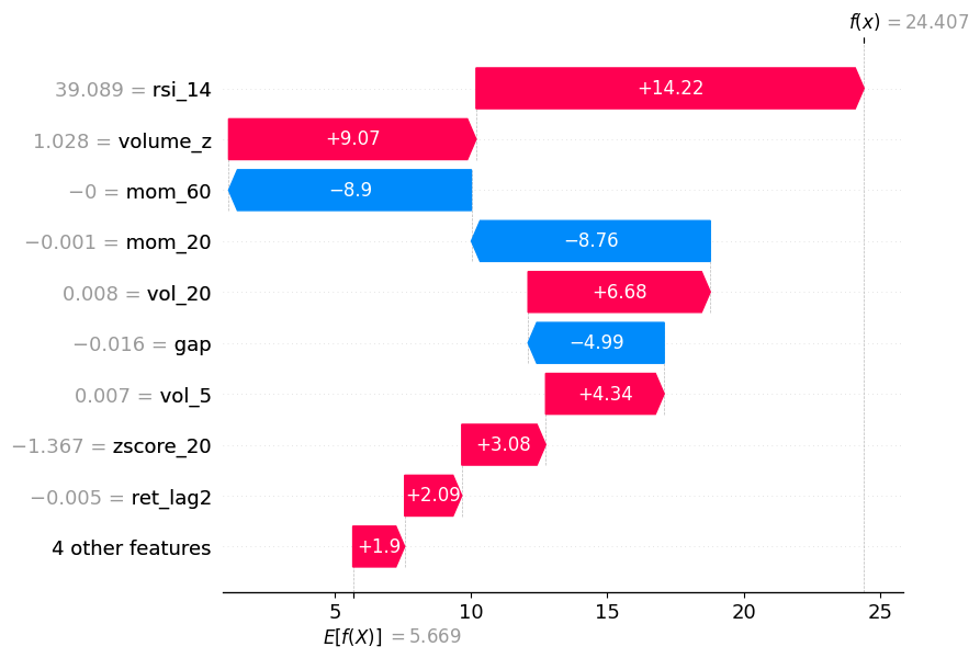
As you can see, momentum pushed the prediction in one direction, but volume_z and RSI pushed it back in the other direction.
force_plot:
Same information as waterfall, but horizontal.
shap.initjs()
shap.force_plot(sv_bps[obs_idx])
decision_plot:
Also gives the same information by showing the cumulative sum of SHAP values as a path from the baseline E[f(.)] to the final prediction.
shap.decision_plot(explainer.expected_value, shap_values[obs_idx].values, X.iloc[obs_idx])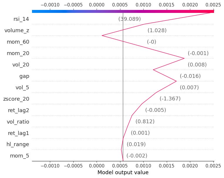
You can also pass multiple observations to compare them side by side:
shap.decision_plot(explainer.expected_value, shap_values.values[:50], X.iloc[:50])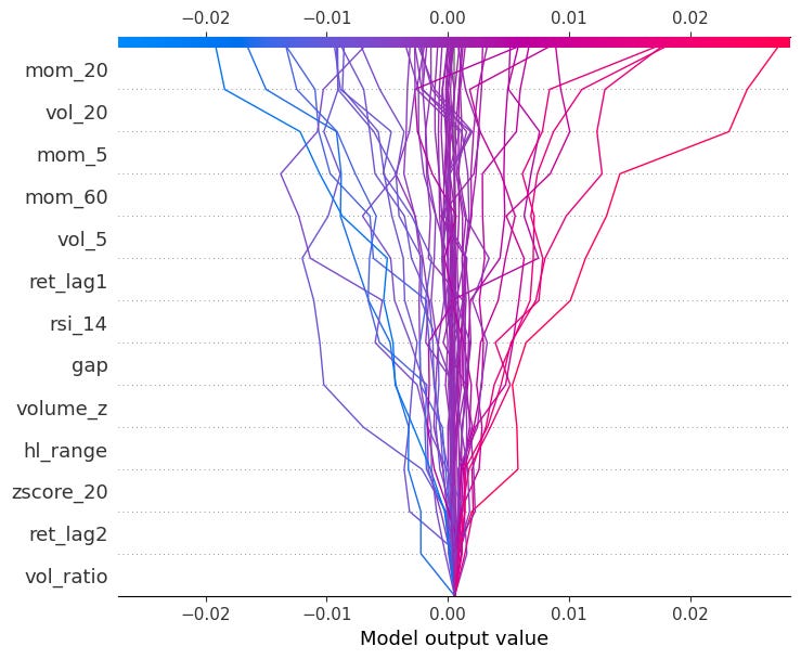
We will get back to SHAP again when looking at global model-agnostic methods!
2. Global Model-agnostic Methods
Global methods answer a different question: not why did the model predict this value for this observation, but how does the model behave on average across the entire dataset? Rather than explaining a single prediction, they summarise the overall relationship between features and the target learned by the model.
Example: You’ve trained a return-forecasting model on SPY, and it performs well out of sample. A local method tells you why the model predicted a large positive return on one specific day. But a global method tells you that across all predictions, volatility is the dominant driver, momentum matters mainly in low-volatility regimes, and the overnight gap feature is essentially ignored by the model.
Let’s go over some of the most popular methods.
2.1 Partial Dependence Plot (PDP)
Remember Individual Conditional Expectation (ICE)? PDP is simply the average of all ICE curves. This also means the PDP inherits the main weakness of ICE: It assumes the feature is independent of the others.
Just like with ICE, a centered version also exists. Let’s implement it as a thick line inside our centered ICE plot:
def ice_plot(model, X, feature, color_by=None, centered=False, ref_value=None, n_obs=100, n_points=100):
    sample = X.sample(n_obs, random_state=42).reset_index(drop=True)
    grid = np.linspace(X[feature].quantile(0.01), X[feature].quantile(0.99), n_points)
    if centered and ref_value is not None:
        grid = np.sort(np.append(grid, ref_value))

    fig, ax = plt.subplots(figsize=(9, 4))
    all_preds = []
    for idx in range(len(sample)):
        preds = cp_profile(model, sample, idx, feature, grid)
        if centered:
            ref = ref_value if ref_value is not None else grid[0]
            ref_pred = preds[np.searchsorted(grid, ref)]
            preds = preds - ref_pred
        all_preds.append(preds)
        color = "steelblue"
        if color_by is not None:
            color = "#d62728" if sample[color_by].iloc[idx] > sample[color_by].median() else "#1f77b4"
        ax.plot(grid, preds, color=color, alpha=0.3, linewidth=0.8)

    pdp = np.mean(all_preds, axis=0)
    ax.plot(grid, pdp, color="black", linewidth=2.5, label="PDP")

    if color_by is not None:
        ax.plot([], [], color="#d62728", label=f"{color_by} high")
        ax.plot([], [], color="#1f77b4", label=f"{color_by} low")

    ax.legend(fontsize=9)
    ax.axhline(0, color="black", linewidth=0.8, linestyle="--")
    ax.set_xlabel(feature)
    ax.set_ylabel("Change in predicted return" if centered else "Predicted return")
    ax.grid(True, alpha=0.3)
    plt.title(f"{'c-ICE' if centered else 'ICE'} Plot — {feature}" + (f" | colored by {color_by}" if color_by else ""))
    plt.tight_layout()
ice_plot(model, X, "mom_20", "vol_20", centered=True, ref_value=0)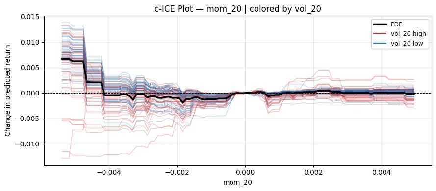
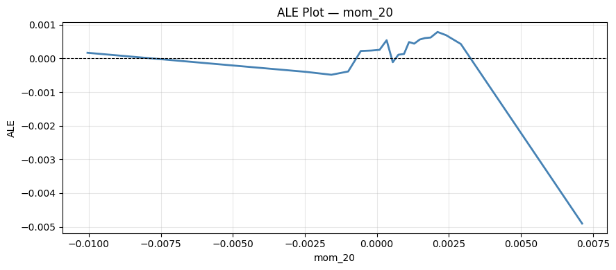
2.2 Accumulated Local Effects (ALE)
PDP’s main weakness is that it sweeps feature x_j across its range while holding other features fixed at their observed values, generating unrealistic feature combinations when features are correlated. ALE fixes this by only looking at the effect of x_j locally, within small neighbourhoods where the feature combinations are realistics, and then accumulating these local effects to get a global picture.
Partition the range of x_j into K intervals [z_{k-1}, z_k]. For each interval, compute the local effect of x_j by averaging the finite difference of predictions over observations that actually fall in that interval:
where K(x) is the index of the inerval containing x, and n_k is the number of observations in interval k. x_{-j}^(i), z_k means that the j-th feature value in x^(i) got replaced with z_k (here i stays for the i-th observation).
Let’s implement this:
def ale_plot(model, X, feature, n_bins=20):
    quantiles = np.quantile(X[feature], np.linspace(0, 1, n_bins + 1))
    quantiles = np.unique(quantiles)

    ale = np.zeros(len(quantiles) - 1)
    bin_centers = np.zeros(len(quantiles) - 1)

    for k in range(len(quantiles) - 1):
        mask = (X[feature] >= quantiles[k]) & (X[feature] < quantiles[k + 1])
        if mask.sum() == 0:
            continue
        X_bin = X[mask].copy()
        preds_high = model.predict(X_bin.assign(**{feature: quantiles[k + 1]}))
        preds_low  = model.predict(X_bin.assign(**{feature: quantiles[k]}))
        ale[k] = (preds_high - preds_low).mean()
        bin_centers[k] = (quantiles[k] + quantiles[k + 1]) / 2

    ale = np.cumsum(ale)
    ale -= ale.mean()

    fig, ax = plt.subplots(figsize=(9, 4))
    ax.plot(bin_centers, ale, color="steelblue", linewidth=2)
    ax.axhline(0, color="black", linewidth=0.8, linestyle="--")
    ax.set_xlabel(feature)
    ax.set_ylabel("ALE")
    ax.grid(True, alpha=0.3)
    plt.title(f"ALE Plot — {feature}")
    plt.tight_layout()
And run it for “mom_20”:
2.3 Friedman’s H statistic
So far, all methods look at the effect of one feature at a time. But in practice, features often interact; the effect of mom_20 on the prediction might be very different in high-volatility vs low-volatility regimes. Friedman’s H-statistic measures the strength of such interactions.
If two features x_j and x_k do not interact, then the point partial dependence can be decomposed as the sum of the individual partial dependences:
The H-statistic measures how much of the joint PDP’s variance is not explained by the sum of the individual PDPs:
H_{jk}^2 is in [0,1], where 0 means no interaction and 1 means the entire joint effect is due to interaction.
There is also a total interaction statistic for feature j measuring its interaction with all other features simultaneously:
Let’s implement both:
from sklearn.inspection import partial_dependence

def h_stat_pairwise(model, X, feat1, feat2, n_samples=500):
    X_s = X.sample(n_samples, random_state=42)

    pd12 = partial_dependence(model, X_s, [feat1, feat2], kind="average", grid_resolution=20)
    pd1  = partial_dependence(model, X_s, [feat1], kind="average", grid_resolution=20)
    pd2  = partial_dependence(model, X_s, [feat2], kind="average", grid_resolution=20)

    grid1 = pd12["grid_values"][0]
    grid2 = pd12["grid_values"][1]
    joint = pd12["average"][0]

    joint -= joint.mean()
    v1 = pd1["average"][0] - pd1["average"][0].mean()
    v2 = pd2["average"][0] - pd2["average"][0].mean()

    numerator, denominator = 0.0, 0.0
    for _, row in X_s.iterrows():
        f12 = joint[np.argmin(np.abs(grid1 - row[feat1])), np.argmin(np.abs(grid2 - row[feat2]))]
        f1  = v1[np.argmin(np.abs(pd1["grid_values"][0] - row[feat1]))]
        f2  = v2[np.argmin(np.abs(pd2["grid_values"][0] - row[feat2]))]
        numerator   += (f12 - f1 - f2) ** 2
        denominator += f12 ** 2

    return np.sqrt(numerator / denominator)

def h_stat_total(model, X, feature, n_samples=500):
    X_s = X.sample(n_samples, random_state=42).reset_index(drop=True)

    f_hats = model.predict(X_s)

    # PD_j: marginalise out all features except j (standard 1D PDP)
    pd_j = partial_dependence(model, X_s, [feature], kind="average", grid_resolution=20)
    grid_j = pd_j["grid_values"][0]
    v_j = pd_j["average"][0]

    # PD_{-j}: for each observation, fix x_{-j} and average over x_j
    pd_minus_j = np.zeros(len(X_s))
    for idx in range(len(X_s)):
        X_temp = X_s.copy()
        X_temp[feature] = X_s[feature]  # vary x_j over training dist
        X_temp.loc[:, [c for c in X_s.columns if c != feature]] = \
            X_s.iloc[idx][[c for c in X_s.columns if c != feature]].values
        pd_minus_j[idx] = model.predict(X_temp).mean()

    numerator, denominator = 0.0, 0.0
    for idx, (_, row) in enumerate(X_s.iterrows()):
        fj    = v_j[np.argmin(np.abs(grid_j - row[feature]))]
        f_hat = f_hats[idx]
        numerator   += (f_hat - fj - pd_minus_j[idx]) ** 2
        denominator += f_hat ** 2

    return np.sqrt(numerator / denominator)
from tqdm import tqdm
import seaborn as sns
features = X.columns.tolist()
h_matrix = np.zeros((len(features), len(features)))
pairs = [(i, j, f1, f2) for i, f1 in enumerate(features) for j, f2 in enumerate(features) if i < j]
for i, j, f1, f2 in tqdm(pairs, desc="Pairwise H"):
h = h_stat_pairwise(model, X, f1, f2)
h_matrix[i, j] = h
h_matrix[j, i] = h
total_h = []
for f in tqdm(features, desc="Total H"):
total_h.append(h_stat_total(model, X, f))
features_sorted, total_h_sorted = zip(*sorted(zip(features, total_h), key=lambda x: x[1]))
fig, axes = plt.subplots(1, 2, figsize=(16, 5))
sns.heatmap(h_matrix, xticklabels=features, yticklabels=features,
annot=True, fmt=".2f", cmap="YlOrRd", ax=axes[0],
linewidths=0.5, cbar_kws={"label": "H-statistic"}, vmin=0, vmax=1)
axes[0].set_title("Pairwise H-statistics", fontsize=13, fontweight="bold")
axes[1].barh(features_sorted, total_h_sorted, color="steelblue")
axes[1].axvline(0, color="black", linewidth=0.8)
axes[1].set_xlabel("H-statistic")
axes[1].set_title("Total H-statistics", fontsize=13, fontweight="bold")
axes[1].grid(True, alpha=0.3, axis="x")
plt.tight_layout()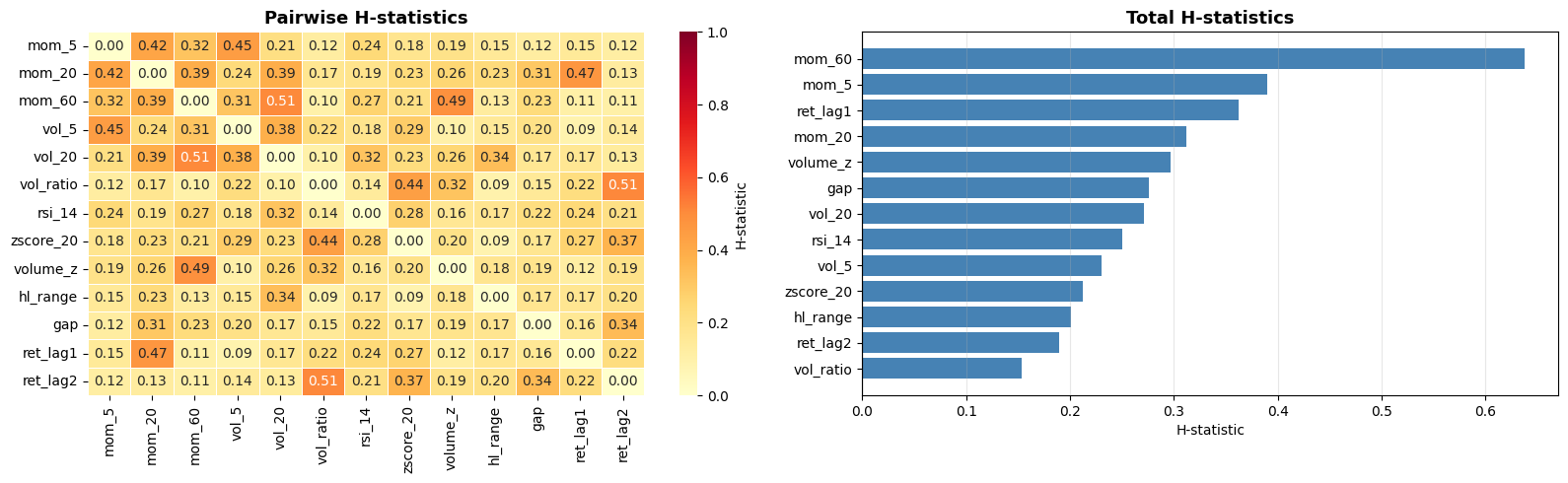
This suffers from the typical drawback of all interpretable machine learning methods: It’s computationally expensive. It also only tells us the strength of the interactions, not what those interactions look like. A good workflow is to measure the interaction strengths with this method and then examine the strongest interactions in more detail using other methods (like specific SHAP plots that we will get to soon).
2.4 SHAP
We already covered how SHAP works so I will only showcase the plots that focus on global effect here.
beeswarm:
Shows the distribution of SHAP values for every feature across all observations.
Each dot is one observation, color indicates the feature value (red=high, blue=low).
Features are sorted by mean absolute SHAP value.
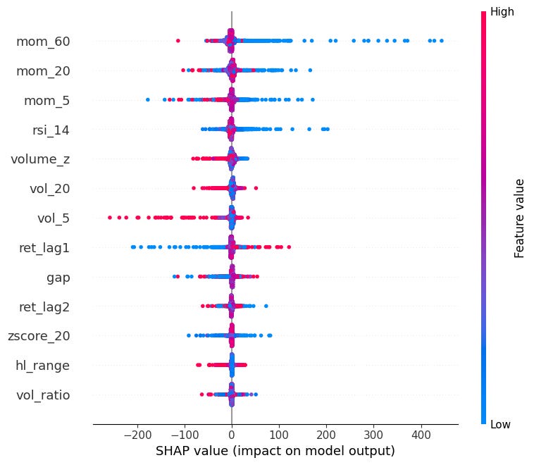
Can see here that very negative momentum causes very SHAP values (mean reversion).
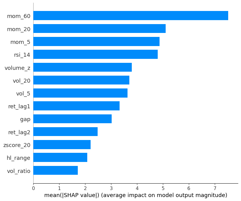
mean absolute SHAP:
Mean absolute SHAP value per feature (global feature importance).
Simpler than beeswarm, good for reporting which features matter most on average.
shap.summary_plot(sv_bps, X, plot_type="bar")
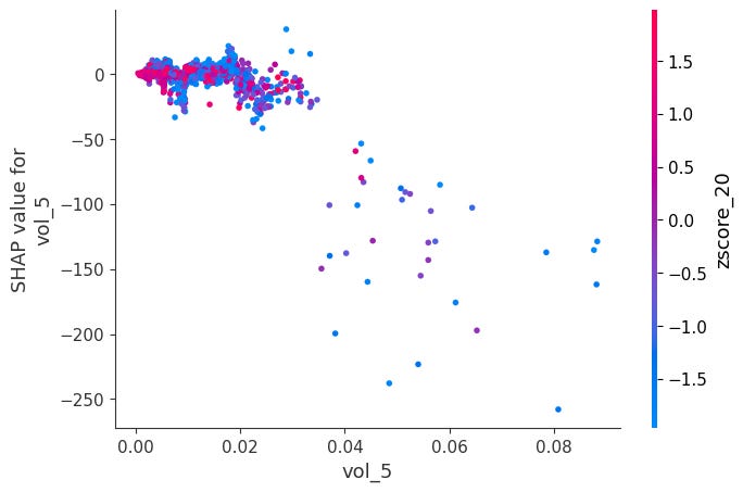
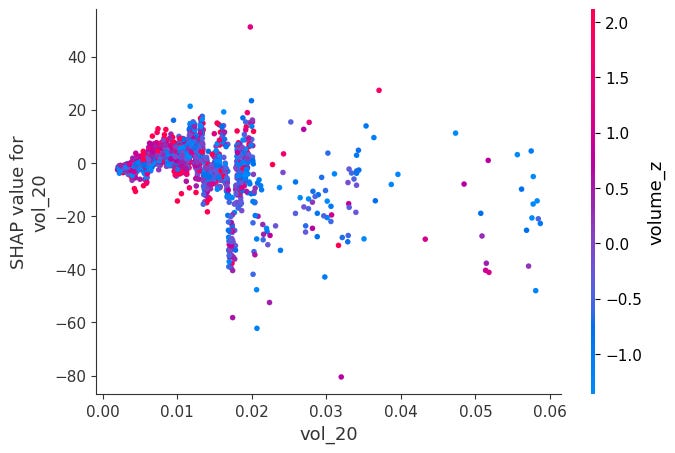
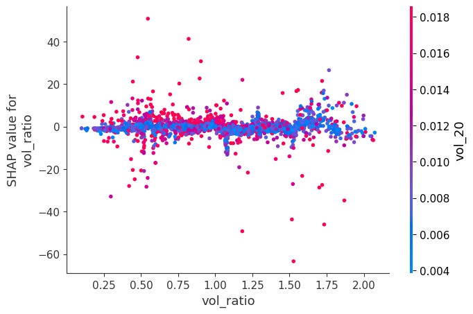
Dependence Plots:
For each feature, it plots phi_j vs x_j across all observations.
Color is automatically chosen as the feature that interacts most with x_j, revealing how the effect of x_j changes depending on another feature's value.
for feat in X.columns:
    shap.dependence_plot(feat, sv_bps.values, X, interaction_index="auto")
Here is a notable ones:
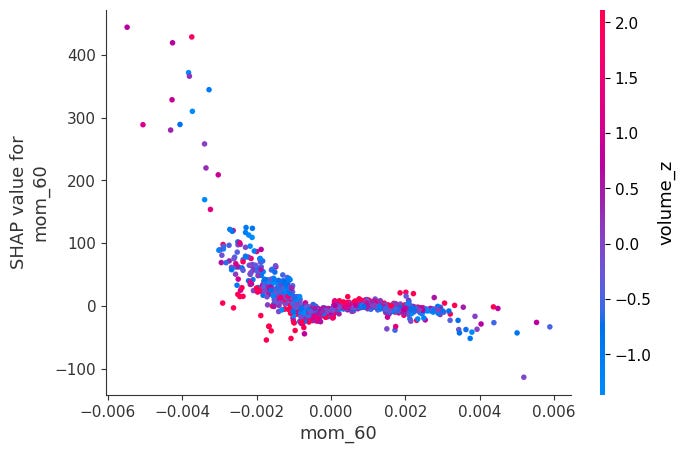
When momentum is very negative and volume is very low, SHAP values become positive. The other ones didn’t have obvious interactions:
Headmap:
Shows phi_j for every feature j and every observation i simultaneously, features as rows and observations as columns. Each cell is colored by the SHAP value: red means the feature pushed the prediction up, blue means it pushed it down.
shap.plots.heatmap(sv_bps)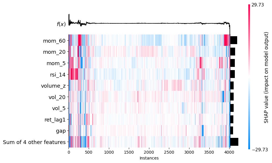
2.5 Permutation Feature Importance (PFI)
We already know about mean absolute SHAP as a general measure of how important a feature is in a model. PFI is another such singular value. If a feature x_j is important, then randomly shuffling its values across observations will destroy its relationship with the target and cause the model’s performance to degrade. If it’s unimportant, shuffling it changes nothing.
We first fit the model and compute a baseline performance metric L (e.g. MSE, R^2, IC) on the dataset. Then, for each feature j, we randomly permute the values of x_j across all observations, leaving all other features unchanged. We recompute the performance metric L^(j) on the permuted dataset, and the importance of feature j becomes
A large Delta L_j means the model relied heavily on x_j, and destroying it hurt performance a lot.
Since permutation is random, it’s standard to repeat this K times and average:
This is much faster to compute than SHAP and is directly tied to model performance, which is what we ultimately care about.
One BIG disadvantage is that if two features are highly correlated, then shuffling one leaves the other intact, and therefore both will receive a lot of permutation importance, even if they are super important to the model performance.
from sklearn.inspection import permutation_importance

result = permutation_importance(model, X, y, n_repeats=30, random_state=42, scoring="r2")

sorted_idx = result.importances_mean.argsort()

fig, ax = plt.subplots(figsize=(8, 5))
ax.barh(X.columns[sorted_idx], result.importances_mean[sorted_idx],
        xerr=result.importances_std[sorted_idx], color="steelblue", capsize=3)
ax.axvline(0, color="black", linewidth=0.8)
ax.set_xlabel("Mean decrease in $R^2$")
ax.set_title("Permutation Feature Importance", fontsize=13, fontweight="bold")
ax.grid(True, alpha=0.3, axis="x")
plt.tight_layout()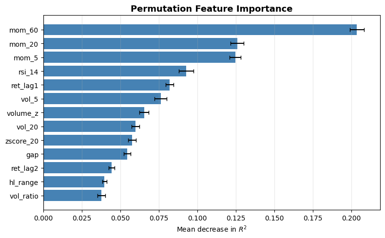
2.6 Leave One Feature Out (LOFO) Importance
Instead of permuting a feature and evaluating with the same model, we completely drop a feature and retrain the model without it. LOFO Importance then measures the performance drop compared to the full model:
This is extremely useful for feature selection, but it is incredibly expensive and suffers from the same issue that highly correlated features get low LOFO importance. If you remove features one at a time, that problem becomes less relevant, as when one of them drops, the other increases in importance and won’t be dropped again.
Let’s implement this with R^2 as our performance metric:
from sklearn.metrics import r2_score

baseline = r2_score(y, model.predict(X))

loo_importance = {}
for feat in tqdm(features, desc="LOO"):
    X_loo = X.drop(columns=[feat])
    m = XGBRegressor(n_estimators=300, max_depth=4, learning_rate=0.05,
                     subsample=0.8, colsample_bytree=0.8, random_state=42)
    m.fit(X_loo, y)
    loo_importance[feat] = baseline - r2_score(y, m.predict(X_loo))

sorted_feats, sorted_vals = zip(*sorted(loo_importance.items(), key=lambda x: x[1]))

fig, ax = plt.subplots(figsize=(8, 5))
ax.barh(sorted_feats, sorted_vals, color="steelblue")
ax.axvline(0, color="black", linewidth=0.8)
ax.set_xlabel("Decrease in $R^2$")
ax.set_title("Leave-One-Out Feature Importance", fontsize=13, fontweight="bold")
ax.grid(True, alpha=0.3, axis="x")
plt.tight_layout()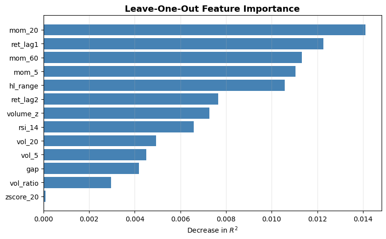
3. Conclusion
I’ve never really written about ML before. If you enjoyed this article and would like to read more about ML, please let me know!
Join Quant Corner: https://discord.gg/X7TsxKNbXg
If you enjoyed this article, please share it!
If you want to read more, consider subscribing!