
The Effective Number of Tested Strategies
A correlation-aware correction for multiple testing in strategy research

In one of my recent articles, we looked at a paper that proposed a measure of how many strategies you effectively tested in-sample. I found the idea of such a measure really interesting and useful, so I went deeper into it, uncovered problems with existing measures, and ultimately came up with my own measure that has all the properties I desire from such a measure!
What is the point of such a measure?
Let’s say you are testing a moving-average crossover strategy, and you test 20 different combinations of moving-average lookbacks. Even for different parameter settings, the strategy returns will be correlated, so you didn’t really test 20 different strategies.
Let’s now dive into ways of measuring this and why it’s incredibly useful.
I write about quantitative trading the way it’s actually practiced:
Robust models and portfolios, combining signals and strategies, understanding the assumptions behind your models.
More broadly, I write about:
Statistical and cross-sectional arbitrage
Managing multiple strategies and signals
Risk and capital allocation
Research tooling and methodology
In-depth model assumptions and derivations
What you’ll learn:
Why the raw number of tested strategies dramatically overstates overfitting risk.
Why dependence geometry determines multiple-testing complexity.
How expected chi-squared maxima define a continuous effective number of tests.
How to compute K_eff numerically.
The 5 Axioms
If I think of a measure of how many strategies were effectively tested, I think of a few intuitive axioms that such a measure should follow:
1 <= K_eff <= K: You can’t test fewer than one strategy, and you can’t test more strategies than you’ve actually tested.
K_eff = 1 iff all strategies are perfectly correlated/anticorrelated: If all your strategies are perfectly correlated/anticorrelated, then you’ve effectively only tested a single strategy.
K_eff = K iff all strategies are uncorrelated: If all your strategies are perfectly uncorrelated (or independent, which is the same in the Gaussian world), then you can’t get more information; you really tested as many strategies as you got.
K_eff is non-decreasing in K: If we test more strategies, our effective number of strategies that we tested can’t decrease; it should only increase, or stay constant if the new strategy is perfectly correlated/anticorrelated to a previously tested strategy.
The expectancy of the maximum of the absolute Z-scores of your K strategies grows asymptotically like the square root of twice the logarithm of K_eff: Okay, this one may not be so intuitive… Let me explain! Let Z_i be the Z-score of strategy i. We assume the Z’s to be standard Gaussian random variables with covariance matrix Sigma. A standard result in extreme value theory is that:
\(\mathbb{E}[\max_{1\leq i \leq K} |Z_i|] \sim \sqrt{2 \log K}\)We want K_eff to be defined so that your correlated portfolio of K strategies looks exactly like K_eff independent strategies in terms of expected best absolute Z-score.
Why Popular Measures Fail
I’m not the first one to come up with a notion of “effective number of strategies tested”, so let’s look at some of the existing definitions and where they ultimately break down.
Spectral Participation Rate
Spectral Participation Rate is the measure that was used in the following article:

It’s defined as follows:
where λ_1, …, λ_K are the eigenvalues of Sigma, which is the correlation matrix of our Z-scores.
By construction, K_eff = K under independence and decreases toward 1 as configurations become collinear. And there you have your problem, K_eff decreases toward 1 as configurations become collinear. Let’s say you have strategies A and B, which are completely independent, so K_eff = 2. Now imagine you were to test strategy B over and over again. You would want K_eff to stay 2, but something else happens.
If you keep adding copies of strategy B, your correlation matrix becomes:
The eigenvalues of Sigma are:
So:
And as K goes to infinity, K_eff converges towards 1!
While this is an extreme example, it happens in reality with adaptive search as well. In Bayesian optimization, you explore parameter areas that previously gave you good results more thoroughly, which in turn gives you a highly correlated strategy and causes K_eff to decrease.
Axiom 4 is clearly violated, and thus, this is not usable for us.
Effective Rank
Effective rank is defined in Roy & Vetterli (2007), and measures effective dimensionality by providing a real-valued extension to the rank of a matrix.
Consider the singular value decomposition (SVD) of Sigma:
where U and V are unitary matrices, and D is a diagonal matrix containing the singular values
Let the singular value distribution be
where sigma is the vector of singular values and ||.||_1 the l1-norm.
The effective rank of the matrix Sigma is defined as
where H is the Shannon entropy given by
We will use this effective rank as our K_eff.
Consider again the scenario of independent strategies A and B, and testing strategy B over and over again. Since Sigma is SPD, the eigenvalues and singular values are the same:
The l1 norm is:
And the singular value distribution is:
With this, erank(Sigma), or K_eff, becomes
This suffers from the same problem as the spectral participation rate! The problem is that those two measures only look at the shape of the spectrum, not its scale. Adding more copies of B drowns out the contribution of A in the normalized distribution, pulling K_eff towards 1.
Bailey & López de Prado
In the paper "The Deflated Sharpe Ratio: Correcting for Selection Bias, Backtest Overfitting and Non-Normality", Bailey and López de Prado present another method of measuring the effective number of strategies tested.
They define
where the equal-weighted average pairwise correlation is
Here is an example where this measure also breaks down:
Let A and B be two perfectly anti-correlated strategies. Then
and the average pairwise correlation is -1.
We get
With this definition, our effective number of strategies tested is 5, even though we only tested 2 strategies. It also violates a bunch of other axioms.
A Definition That Works
Here is what I propose. Let M(x) be the expected maximum of x i.i.d. squared standard normal random variables:
Equivalently, since squaring a standard normal random variable yields a chi-squared random variable, this is the expected maximum of x i.i.d. chi-squared random variables. Using the PDF and CDF, we write the expected maximum as:
M is strictly increasing and continuous, so it has a well-defined inverse
We then define the effective number of tested strategies as:
where Z_1, …, Z_K are the actual strategy Z-scores with correlation matrix Sigma. In other words, K_eff is the number of independent strategies that would produce the same expected best squared Z-score as your actual correlated portfolio of K strategies.
Now, let’s prove that this definition actually follows the 5 axioms.
Axiom 1
Since M is strictly increasing, it suffices to show that
Lower bound:
Upper bound:
By Šidák’s inequality for centered Gaussian vectors,
Since each Z_i is standard normal, we have
and hence
where st means stochastically dominated. And because x → x^2 is increasing,
Taking expectations gives
Axiom 2
If all strategies are perfectly correlated or anticorrelated, then for every i,j,
Since each Z_i is standard Gaussian, this implies there exists a single standard normal random variable X and signs epsilon_i, either -1 or 1, such that
Therefore,
so
Taking expectations,
Applying the inverse of M,
Now the other direction. Assume K_eff = 1. Since M(1) = 1,
Since each Z_i is standard Gaussian, we have E[Z_i^2] = 1.
Since
the equality
can occur only if
Thus
For jointly Gaussian variables, this implies
and therefore
Axiom 3
If all strategies are uncorrelated, we have
which implies that
Therefore,
Applying the inverse of M, we get
Now the other direction. Assume K_eff = K. Since M is strictly increasing,
Now let
From the proof of Axiom 1, we know that
i.e.
Using the tail-integral formula,
The integrand is nonnegative everywhere, and the left-hand side is zero since E[X] = E[Y]. Hence
Thus, X and Y have the same distribution. Equivalently,
By the equality case of Šidák’s inequality, this implies that Z_1, …, Z_K are independent, which for Gaussian random variables is equivalent to being uncorrelated.
Axiom 4:
We have
Taking expectation
and applying the inverse of M, we get
Axiom 5:
Let
Then
A standard result from Gaussian extreme-value theory states that
Moreover,
is uniformly integrable. Hence, convergence in probability implies convergence of expectations:
Hence
Substituting k = K_eff yields
Since
we obtain
Since Gaussian maxima concentrate sharply, the first and second moments are asymptotically equivalent up to square-root scaling. Therefore,
Simulation
Below is the code used for computing K_eff:
import numpy as np
from scipy.stats import chi2
from scipy.optimize import brentq


def M(x: float, n_quad: int = 4000) -> float:
    """
    Compute M(x) = E[max of x i.i.d. chi^2_1 variables] via numerical
    quadrature, working in log space to avoid underflow.

    Parameters
    ----------
    x       : effective count (any real >= 1)
    n_quad  : number of quadrature points

    Returns
    -------
    float : E[max_i Z_i^2] for x i.i.d. N(0,1) variables
    """
    # Adaptive upper limit: tail of chi^2_1 maximum decays beyond this
    hi = chi2.ppf(1 - 1e-10 / x, df=1) if x > 1 else chi2.ppf(1 - 1e-8, df=1)
    t  = np.linspace(0, hi, n_quad + 1)[1:]  # avoid t=0 where pdf diverges

    log_F   = chi2.logcdf(t, df=1)
    log_f   = chi2.logpdf(t, df=1)
    log_ker = np.log(t) + np.log(x) + log_f + (x - 1) * log_F

    # Zero out terms that underflow (negligible contribution)
    mask       = log_ker > -700
    integrand  = np.zeros_like(t)
    integrand[mask] = np.exp(log_ker[mask])

    return float(np.trapezoid(integrand, t))


def M_inv(val: float, tol: float = 1e-8) -> float:
    """
    Compute M^{-1}(val) via Brent's method.

    Parameters
    ----------
    val : target value, must be >= M(1) = 1
    tol : tolerance for root finding

    Returns
    -------
    float : x such that M(x) = val
    """
    if val <= 1.0:
        return 1.0

    # Bracket: expand upper bound until M(hi) > val
    hi = 2.0
    while M(hi) < val:
        hi *= 2.0

    return brentq(lambda x: M(x) - val, 1.0, hi, xtol=tol)


def K_eff(Sigma: np.ndarray, n_sim: int = 200_000, seed: int = 42) -> float:
    """
    Compute K_eff for a portfolio of K strategies with correlation matrix Sigma.

    Uses Monte Carlo to estimate E[max_i Z_i^2], then inverts M analytically.

    Parameters
    ----------
    Sigma : (K, K) correlation matrix
    n_sim : number of Monte Carlo samples
    seed  : random seed

    Returns
    -------
    float : K_eff in [1, K]
    """
    K   = Sigma.shape[0]
    rng = np.random.default_rng(seed)
    L   = np.linalg.cholesky(Sigma)
    Z   = (L @ rng.standard_normal((K, n_sim)))  # (K, n_sim)
    E_max_Z2 = float(np.mean(np.max(Z**2, axis=0)))
    return M_inv(E_max_Z2)
And now let’s simulate how K_eff evolves as K grows for different families of strategies:
import matplotlib.pyplot as plt


# ============================================================
# Helper: build equicorrelation matrix
# ============================================================

def equicorr_matrix(K, rho):
    """
    Build K x K equicorrelation matrix with off-diagonal rho.
    """

    Sigma = np.full((K, K), rho, dtype=float)
    np.fill_diagonal(Sigma, 1.0)

    return Sigma


# ============================================================
# Sequential simulation
# ============================================================

def sequential_keff(mode, K_max=100):

    K_vals    = []
    Keff_vals = []

    # Persistent storage for sequential random strategies
    random_vectors = []

    rng = np.random.default_rng(123)

    for K in range(1, K_max + 1):

        # ----------------------------------------------------
        # Independent
        # ----------------------------------------------------
        if mode == "independent":

            Sigma = np.eye(K, dtype=float)

        # ----------------------------------------------------
        # Perfect dependence
        # ----------------------------------------------------
        elif mode == "dependent":

            Sigma = np.ones((K, K), dtype=float)

        # ----------------------------------------------------
        # rho = 0.5
        # ----------------------------------------------------
        elif mode == "rho_0.5":

            Sigma = equicorr_matrix(K, 0.5)

        # ----------------------------------------------------
        # Maximally negative equicorrelation
        # ----------------------------------------------------
        elif mode == "negative_boundary":

            if K == 1:
                rho = 0.0
            else:
                # PSD boundary:
                # rho >= -1/(K-1)
                rho = -0.9 / (K - 1)

            Sigma = equicorr_matrix(K, rho)

        # ----------------------------------------------------
        # Sequential random correlated strategies
        # ----------------------------------------------------
        elif mode == "random":

            # Add ONE new latent-factor strategy
            v = rng.standard_normal(5)

            # Normalize
            v /= np.linalg.norm(v)

            random_vectors.append(v)

            X = np.stack(random_vectors)

            # Correlation matrix
            Sigma = X @ X.T

        else:
            raise ValueError(f"Unknown mode: {mode}")

        # ----------------------------------------------------
        # Numerical stabilization
        # ----------------------------------------------------

        Sigma = Sigma.astype(float)

        Sigma += 1e-10 * np.eye(K)

        # ----------------------------------------------------
        # Compute K_eff
        # ----------------------------------------------------

        keff = K_eff(Sigma)

        K_vals.append(K)
        Keff_vals.append(keff)

        print(
            f"{mode:20s} | "
            f"K = {K:3d} | "
            f"K_eff = {keff:8.3f}"
        )

    return np.array(K_vals), np.array(Keff_vals)


# ============================================================
# Run all simulations
# ============================================================

modes = [
    "independent",
    "dependent",
    "rho_0.5",
    "negative_boundary",
    "random"
]

results = {}

for mode in modes:

    K, Keff = sequential_keff(mode, K_max=100)

    results[mode] = (K, Keff)


# ============================================================
# Plot
# ============================================================

plt.figure(figsize=(12, 8))

for mode in modes:

    K, Keff = results[mode]

    plt.plot(K, Keff, linewidth=2, label=mode)

# Reference line
plt.plot(
    np.arange(1, 101),
    np.arange(1, 101),
    linestyle="--",
    linewidth=2,
    label="K_eff = K"
)

plt.xlabel("Raw Number of Tested Strategies (K)")
plt.ylabel("Effective Number of Strategies (K_eff)")

plt.title(
    "Sequential Growth of K_eff Under Different Correlation Structures"
)

plt.legend()
plt.grid(True)

plt.show()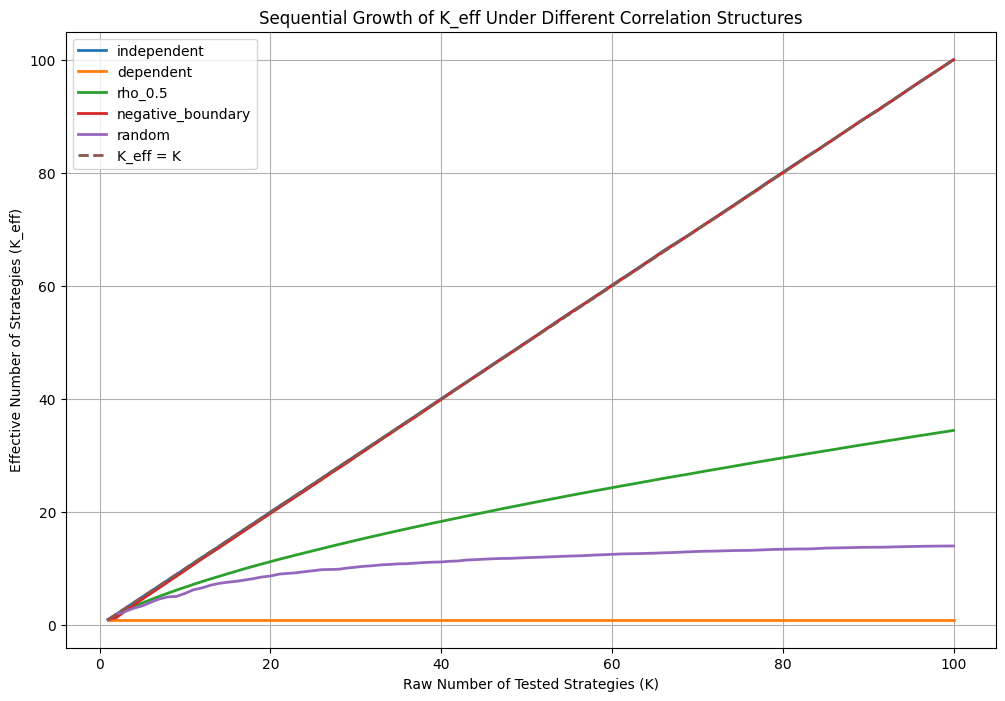
Conclusion
K_eff is not just theoretical; it has immediate practical applications.
The most direct one is improving the Deflated Sharpe Ratio presented by Bailey and De Prado. More broadly, K_eff can be used anywhere you need to correct for multiple testing across correlated strategies.
It can also directly guide you in determining when to stop searching while tuning hyperparameters.
I will explore those and many other things K_eff is capable of, and the math behind K_eff in more detail in future articles, which I then plan to all combine into a research paper!
Join Quant Corner: https://discord.gg/X7TsxKNbXg
Quick reminder that I’m now open for consulting and short-term engagements. If your team needs help with anything in the quant space, like strategy research, portfolio construction, execution analysis, signal development, or just a second brain on a hard problem, I'm available. You can DM me on Discord or email me at vertoxquant@gmail.com.